Streams July 27 and July 29 2024
Streams July 27 and July 29 2024
Note: This notebook was made on a livestream, and so not everything is written in stone or thoroughly fact checked!
Keep in mind that it’s meant as a record of what we did on stream and a repository of source code, so it’s not a pedagogically sound well-written document!
Keep in mind that it’s meant as a record of what we did on stream and a repository of source code, so it’s not a pedagogically sound well-written document!
Old code + Description of what I’m trying to do
Old code + Description of what I’m trying to do
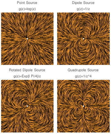
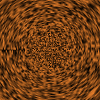
The starting points are these images, coded in late 2022. This notebook is all about the work involved in animating them!
Out[]=
The images visualize flow fields. So they’re best interpreted as orange particles moving on the surface of water, with a motion blur filter applied to the picture. SO the obvious thing to do would be to let the particles move over time and animate it that way. Unfortunately this will require a lot of work!
P.S. Expand the image cell above see the code that generates them.
Other fluid flow stuff:
Other fluid flow stuff:
If we want to find the position of the orange particles as a function of time, we could use the same formulas used in Aubrey Jaffer’s webpage on fluid marbling patterns. https://people.csail.mit.edu/jaffer/Marbling/Mathematics . But I’m going to do this from scratch + explore!
In[]:=
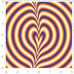
V=1.0;L=0.2;scalarFunction[{x_,y_}]=Sin[Sqrt[x^2+y^2]10];strokeTransform[{x_,y_}]={x,y+VExp[-Abs[x]/L]};wavyTransform[{x_,y_}]={x+0.05y^2,y};wavyTransformInverse[{x_,y_}]=({x2,y2}/.Solve[Thread[wavyTransform[{x2,y2}]=={x,y}],{x2,y2}][[1]]);Rasterize[DensityPlot[scalarFunction[wavyTransformInverse[strokeTransform[wavyTransform[{x,y}]]]],{x,-3,3},{y,-3,3},MaxRecursion->5],ImageSize->{256,256},Background->Transparent]
Out[]=
First pass at new code
First pass at new code
Making a Translating Image
Making a Translating Image
First, let’s just get a translating image which uses the same orange and black color scheme:
In[]:=
width=64;height=64;color[t_]={0,0,0}t+(1-t)List[0.91,0.5,0.17];ClearAll[translatedImage];baseArray=Table[color@RandomReal[],{j,1,height},{i,1,width}];translatedImage[amount_]:=translatedImage[amount]=Image[RotateRight[#,amount]&/@baseArray];
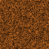
We get a translating random orange and black image:
In[]:=
Manipulate[translatedImage[k],{k,1,width,1}]
Embedded gif for viewing on the Wolfram cloud:
Gif generating code
Gif generating code
Passing them into Line Convolution
Passing them into Line Convolution
To start with, let’s just use these frames as input to LineConvolutionPlot. It won’t end up generating good results, but it’s a start.
In[]:=
g[z_]=Log[z];nframes=2;imgTableFirstPass=Table[LineIntegralConvolutionPlot[{Re[Grad[g[z]/.zx+yI,{x,y}]],translatedImage[Floor[widthframe/nframes]]},{x,-1,1},{y,-1,1},EvaluatedTrue,FrameFalse,ImageSize64],{frame,0,nframes-1}];//AbsoluteTiming
Out[]=
{15.6814,Null}
With just two frames it’s hard to tell what’s going on in the animation:
In[]:=
Row[imgTableFirstPass]
Out[]=
But with the full .gif it’s easier to see what’s going on, and it’s easy to see that passing a translating image into the LineIntegralConvolutionPlot function doesn’t do what we want!
Trying something else!
Trying something else!
Any approach like this will just result in boring translations.
So I have to use the formulas that Jaffer uses: https://people.csail.mit.edu/jaffer/Marbling/Mathematics
A few approaches to figuring this out...
So I have to use the formulas that Jaffer uses: https://people.csail.mit.edu/jaffer/Marbling/Mathematics
A few approaches to figuring this out...
◼
Work out the transformations by hand (something
likez(t)=+2it
2
z
0
◼
Try it a hacky way first
The Hacky Way:
The Hacky Way:
So like I said at the start, the ideal animation would be one that actually tracks the motion of fluid particles over time. We’re not gonna do that, we’re just going to try something that tries to fake the animation.
I’m going to start by trying to animate this image:
Let’s just do a hacky way by doing a coordinate transformation that looks like the following. I transform the pixel image from square coordinates like on the left, to cylindrical coordinates like on the right:
Out[]=
↦
I’m using the ImageTransformation command. The texture on the left is indexed by coordinates with being the top left and being the bottom right. I want to define a map such that... (the left side of the image gets mapped to the center of the new image) (the right side gets mapped to a circle)To figure out the constant, we have to decide on const =
(u,v)
(0,0)
(1,a)
(0,v)|->(0.5,0.5)
(1,v)|->(0.5,0.5)+1(Cos[const*v],Sin[const*v])
(1,0)|->(0.5,0.5)+1(1,0)
(1,a)|->(0.5,0.5)+1(Cos[const*a],Sin[const*a])
2π
a
The forward transformation is this:
In[]:=
forwardTransform=({1,a}/2+#[[1]]{Cos[#[[2]]2Pi/a],Sin[#[[2]]2Pi/a]})&
ImageTransform needs the inverse of this transformation, and that’s going to be a pain to figure out!
Figuring out the inverse transform:
Figuring out the inverse transform:
Note: at the end of the day this is just transforming back and forth between cylindrical and Cartesian coordinates, and I’m really doing it a very dumb way here. This is more of a “using a sledgehammer to crack a walnut” solution.
The inverse transformation is:
Note: ArcTan has a range [-Pi,Pi], so I’m just going to add Pi to it.
If we were thinking deeply about this problem, we could check that this formula is consistent with our requirements for the forward transformation. But let’s skip that and just use the formula!
Getting a simple animation
Getting a simple animation
Still frame:
Embedded gif:
Putting LineIntegralConvolution plot over it:
Putting LineIntegralConvolution plot over it:
So, beforehand we put translating images into LineIntegralConvolutionPlot. Now we’re going to put this expanding animation into LineIntegralConvolution plot. We can try it with different vector fields.
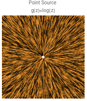
The single source looks quite boring:
Putting an obstacle in the way looks cooler:
A dipole looks the coolest:
Doing it the correct way (?)
Doing it the correct way (?)
Okay, so the cheating way gives us cool images but maybe we should just do it the correct way from the beginning.
We did a bunch of math:
Checking formulas are correct:
Checking formulas are correct:
These two formulas should be equivalent:
Equation on the righthand side says:
So we’ve proved that the equation is correct, in general it looks like we’ll have nasty implicit functions in the solution.
^ IMO this demonstrates that we’re not going to get useful formulas in an easy way!
Key takeaway
Key takeaway
Revert to numerics the only option?
I guess so! Time to implement things in Shadertoy or experiment with specific setups in Mathematica, but I can’t do a fast and general render in Mathematica.
The correct way but for a specific case
The correct way but for a specific case
I can’t end it there! We didn’t solve for a general g, but let’s at least make a plot solving for the g=log(z) case. This section is very hacked together code. I just wanted to get something done!
So we have a function that maps {x,y} to some other point {x(t),y(t)}.
We have a point {x,y} and a time t and we have to decide on a color.
{x,y} should take its color from F[x,y,t].
We have a point {x,y} and a time t and we have to decide on a color.
{x,y} should take its color from F[x,y,t].
Let’s use a funny image for our input:
Tangents
Tangents
Making a gallop sound in Mathematica
Making a gallop sound in Mathematica
I mentioned that the MIDI sounds in Mathematica are really good now, for example we can make a gallop pretty easily. In this very quick example, “b” is short for “beat”, “r” is short for “rest”, and “h” is short for “high”.
Viewer Question: When does a^m make sense for square matrix m?
Viewer Question: When does a^m make sense for square matrix m?
Some scratchwork related to that:
Some scratchwork related to that:
Recall the identity:
Writing the matrix expressions:
Checking for 2 to the identity matrix.
Checking for 2 to the 2x2 matrix of ones:
Checking for 2 to the {{0,1},{-1,0}}:
Another fun idea: Can we make a QR code out of the flow field images?
Computational physics portfolio project:
Computational physics portfolio project:
mewondering6’s question: what should i do, what projects, languages, should i analyze the job market and learn the language that is most asked for?
My answer: It’s highly dependent and I’m not quite the best person to ask, but I can certainly suggest good projects!
One good project is this beautiful wave simulator project by 0x23: https://github.com/0x23/WaveSimulator2D
My answer: It’s highly dependent and I’m not quite the best person to ask, but I can certainly suggest good projects!
One good project is this beautiful wave simulator project by 0x23: https://github.com/0x23/WaveSimulator2D
The code is really short, the updating of the image is done in six lines of Python! (handled in update_field in source/wave_simulation.py)
Nils Berglund, who has similar projects but written in C, also posts his source code publicly: https://www.youtube.com/watch?v=-RJ0Y1EDJZY
dr_cook_’s recommendations and Clifford algebra stuff
dr_cook_’s recommendations and Clifford algebra stuff
Animating Spherical Harmonics
Animating Spherical Harmonics
We got distracted talking about nice animations of something like hydrogen atom orbitals. White this isn’t exactly a hydrogen atom orbital, this is still a very cool project and it can be done very quickly.
First I define random sums of spherical harmonics, and I superimpose three wavefunctions on the sphere with frequencies of 1, 1/2, and 1/3. (So the total period is T=2*pi*lcm(1,2,3)=12*pi):
Then I define a plot function. These options are my preferred way of animating! SphericalRegion would be especially important if we wanted the camera to circle around the rotating ball, but with a stationary camera I suppose it isn’t necessary. Likewise I ignore ColorFunctionScaling, we can do all of our color function scaling ourselves.
And finally, outputting a .gif:
“DisplayDurations” can also accept a list argument:
Combining the frames into a cool table:
Combining the frames into a cool table:
Combining the frames in a cool way:
Stylesheet Work
Stylesheet Work
Dark mode
Dark mode
For stream, I use the dark mode stylesheet by Jakob Neef: https://gitlab.com/jakobneef/mathemeatica
Removing the stylesheet at the end of the day:
Thinking about gif embedding:
Thinking about gif embedding:
Manipulate is too annoying to get working on the web
ListAnimate works but has huge filesizes
So I guess I’ll just WebEmbed .gifs for everything.
ListAnimate works but has huge filesizes
So I guess I’ll just WebEmbed .gifs for everything.
Next Stream Idea:
Next Stream Idea:
Implement Bells of Bezelea using SoundNote: https://pub.colonq.computer/~bezelea/bells/index.html
Talking with dr_cook_:
Minutephysics visualization using Blender + atomic orbital irreps (writing to .blend files from Mathematica would be easy... right?)
Illustrations of river coordinates (Gullstrand-Painleve)
Get code working to easily create small .gifs and compress them.
Talking with dr_cook_:
Minutephysics visualization using Blender + atomic orbital irreps (writing to .blend files from Mathematica would be easy... right?)
Illustrations of river coordinates (Gullstrand-Painleve)
Get code working to easily create small .gifs and compress them.
What did we accomplish this stream:
What did we accomplish this stream:
Organization work on the July 27th stream,
Figured out how to embed .gifs in web notebooks,
Experimented with .gif creation,
Met some people + got some ideas for future streams (more spherical harmonics, minutephysics visualizations, exporting to Blender from mathematica)
Figured out how to embed .gifs in web notebooks,
Experimented with .gif creation,
Met some people + got some ideas for future streams (more spherical harmonics, minutephysics visualizations, exporting to Blender from mathematica)
