Characterisation of topological invariants in discrete lattice geometries via graph re-writing
1. GRACYASK (GRAphs CYcles And SKyrmions):
by Sinuhé Perea - Puente (King' s College London)
1. GRACYASK (GRAphs CYcles And SKyrmions):
by Sinuhé Perea - Puente (King' s College London)
2. ABSTRACT: We are going to study finite lattice systems in the context of simple re - writing rules : Based on discrete manifolds and Cayley graphs, in this project we look for the set and taxonomy of simple re - writing rules that preserve certain properties that can later be understood as conserved measurable magnitudes of a physical system, like the Brouwer degree or winding number . By investigating those toy-models about field configurations of discrete fiber bundles, we will later apply local perturbations to a field configuration, looking for discrete analogs to Noether’ s Theorem . Furthermore, via coloured graphs, with this approach we will aim to characterise (energetically stable) physical - inspired systems in the context of many - particle quantum finite distributions in highly symmetric arrays or low - dimensional spin - like states as domain wall in magnetization theory, being local solutions of minimal information configurations . Even mesoscopic scale is responsible for exotic topological defects, with this discretization we will try to understand the computational first - principle mechanism that allows non - trivial winding numbers and the material and geometries to host pseudo - particle structures like skyrmions, bubbles or merons . We think that this inductive reasoning here would offer a valuable approach for finding new phenomena or even re - interpreting old ones .
3. Motivation
3. Motivation
In several physics systems the whole can be obtained as an exact copy of each of its parts, which facilitates the study of a complex system by looking carefully at its elements, separately. Reductionism offers simplified models which makes the problems easier, but “there’s plenty of room...at the discrete scale”. Here we present a tour for two of its representants: Quivers and skyrmions, studying some of its basic definitions and properties, and an example where both arise together.
For that, we are going to primarily use the quiver module for Mathematica by Taliesin Beynon. Available at https://github.com/taliesinb/QuiverGeometry, and carefully developed in https://quivergeometry.net.
4. Introduction: A new (space) hole
4. Introduction: A new (space) hole
4.1.-Start here: To read/run only the first time
4.1.-Start here: To read/run only the first time
tldr: In the following notebook tries to be a illustrative tutorial for showing some results in simple discrete lattice geometries. In principle all the output sections are displayed so unless you want to play around I don’t recommend to run them again, because some of them takes some time to fully proceed (they are marked with the comment *IDLE*)
First of all, if you get ANY instability during the execution, run the following code:
In[]:=
Quit[]
If you want to interact with this notebook, you will need to download the GitHub repository “quivergeometry”and clone it in your local machine. Then you need to import the module via introducing the directory of the file “init.m”:
In[]:=
Get["C:\\Users\\k20004058\\OneDrive - King's College London\\Documents\\GitHub\\QuiverGeometry\\Kernel\\init.m"] (*Change USERNAME*)
Some initial codes to refresh the kernel:
In[]:=
GenerateQuiverGeometryStylesheet[];ClearBundleData[];GQG;
4.2.-Basic tools: Quiver structures
4.2.-Basic tools: Quiver structures
Our basic construct will be quiver functions that represent base (B) and fibre (F) spaces, being the total space the Cartesian product of the previous .
E:B×F
With the addition of a map , we can form a bundle as the triplet Some examples of basis, trivial (when the map is a projection in the first component) and non trivial bundles are the following:
π:E->B
(E,π,B)
In[]:=
MatrixForm[{"Increasing size of the quiver geometries->","Linear (Z)"->Table[LineQuiver[n,ImageSize->115],{n,4,5}],"Cyclic/periodic (Zn)"->Table[CycleQuiver[n],{n,3,5}],"Triangular"->Table[TriangularQuiver[n,ImageSize->70],{n,2,4}],"Cubic"->Table[CubicQuiver[n,ImageSize->125],{n,2,3}],"Bundle E=BxF"->TrivialBundleGraph[8,3,ImageSize->230],"Mobius strip"->MobiusStrip[8]}]
Out[]//MatrixForm=
Increasing size of the quiver geometries-> |
Linear (Z){ , } |
Cyclic/periodic (Zn) , , |
Triangular , , |
Cubic   |
Bundle E=BxF |
Mobius strip |


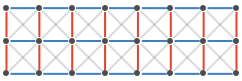
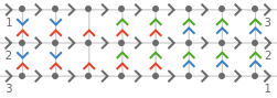
Figure 1.Different examples of quiver geometries: Linear and cyclic bases (1D), triangular (2D), cubic (3D), trivial (×) and non trivial (Möbius strip) bundles.
L
8
L
3
As you may have see here, we are talking about discrete structures, so if we may need to redefine some concepts. When we have defined the spaces, the next step is to find the elements there. The objects for playing will be the graph of functions, represented as a collection of vertices and edges. In this notebook, we are going to consider “smooth”-like discrete functions implying that the connected vertex are only adjacent or in the same fiber section to the previous and following one, or in plain words, you can just go right (through the basis) and one position up, constant o down (through the fiber). We define the set of this elements as . Below you can interact with a trivial linear bundle, and see the different elements in .
1
D
1
D
In[]:=
Manipulate[{TrivialBundleGraph[aa,bb,ImageSize->20*aa],Part[FindAllBundleSections[TrivialBundleGraph[aa,bb,ImageSize->20*aa,SectionDisplayMethod -> dd]],cc]},Style["Linear space"Dynamic[aa]Dynamic[bb], 12, Bold],{{aa,4,"B=Base size"},2,6,1,ImageSize -> Tiny},{{bb,3,"F=Fibre size"},2,5,1,ImageSize -> Tiny},{{cc,Random[Integer,{1,9}],"Field config"},1,Length[FindAllBundleSections[TrivialBundleGraph[aa,bb]]],1,ImageSize -> Tiny},{{dd,"Total","Display"},{"Total","Line","Base","Array"}}]
Out[]=
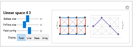
Figure 2.Different trivial linear bundle examples, for different sizes of the base and the fiber (left). “Smooth” section or field configuration for the same bundle (right). Different display options (total/line for showing/hiding the “grid” and array for a full/compact colour base RBGOP...).
In the last section of the notebook, we will introduce some physical examples for this abstract mathematical concept. We can see how we can make the system to “evolve” to go from an initial state to a final state via swapping a single vertex up or down, leading us to define a discrete version of homotopy in which two states are related (they are homotopically equivalent) if we can smoothly deform one into the other. The continuous version from [A] “Given two continuous functions f (x), g(x) defined in their respective topological spaces, both functions are homotopic iff exist a continuous function h(x, t) s.t. h(x, 0) = f (x) and h(x, 1) = g(x)”. Here we can just obtain the discrete version if we can obtain go between both in a finite number of (allowed) steps. And how can we characterise these derived paths? That is exactly the idea of rewriting systems [B].
5. Bundle taxonomy: the rewriting strikes back
5. Bundle taxonomy: the rewriting strikes back
Next question we address then is how can "travel" between different states (this could also potentially lead us to define the neighbourhood of a given element and induce a toy-topology). This will be done introducing the rewriting system graph, that will give us valuable information about the system. We will start by considering a simple case to later start a brief characterisation of some families of bundles, using Cayley graphs.
In[]:=
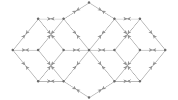
examplegra=TrivialBundleGraph[3,3]; (*Empty total space*)examplebun=FindAllBundleSections[examplegra]; (*All the possible sections*)examplerew=BundleSectionRewritingSystem[examplegra];(*The rewriting system*)examplecay=RewriteGraph[examplerew,Part[examplebun,1],ImageSize->300]RewriteQuiver[BundleSectionRewritingSystem @ examplegra,All,VertexSize->30,VertexShapeFunction->"Vertex"->Function[BundleSectionPlot[#,Method->"Line"]],GraphLegend->Automatic,ImageSize->300]
Out[]=
Out[]=

Figure 3.Rewriting system graph for the bundle × with schematic vertices (top) and explicit description (bottom) with different colours for action of each of the vertices.
L
3
L
3
As you can see above, there is an obvious discrete parity symmetry (we can see left and right parts are quiral, with the mirror inversion), and also we can see that they are common structures between constant bundles (when all the vertices has the same “level”, like the movement of a chess tower). This is related to the concept of connection (in the “Berry phase” sense) under quotient topology and general gauge theory [C], which was more theoretically treated in [D]. An more closer example could be the different branches of the logarithm in complex analysis.
It is also interesting to take the quotient group with this different elements and see that, for example the mirror symmetry behaviour links quiral states, behind the subjacent group , while the connections will allow us to just consider isomorphic copies of the simpler cases (and adding manually some extra objects for the cyclic behaviour from the linear, for instance). Furthermore, it is possible to consider discrete analog to Noether’s Theorem, that will be clearer when the physical image is present, to quotient again the possible states and analyse a smaller set (in particular we will see this in the torus structure with translations along base and fiber spaces). In [E] this idea is discussed in the context of the Ising model. As we can see, this abstract mathematical ideas can have direct corollaries in Physics.
Z
2
These will be the basic ideas we are going to explore below for a general classification of these kind of quiver graphs.
5.1.-Linear quivers
5.1.-Linear quivers
We are going to begging studying the linear quiver where there is no quotient topology (“gluing” of points in the boundaries). First we are going to introduce a couple of families to later discuss the general structure, characterisation and limiting cases. The first case will be the Rubber band, where we are going to introduce the concept of elasticity.
5.1.1.-Linear rubber band: L2×Ln
5.1.1.-Linear rubber band: ×
L
2
L
n
In[]:=
Manipulate[Module[{rubber},rubber=TrivialBundleGraph[2,fib];RewriteQuiver[BundleSectionRewritingSystem @ rubber,All,VertexSize->10*fib,VertexShapeFunction->"Vertex"->Function[BundleSectionPlot[#,Method->dis]],ImageSize->100*fib]],{{fib,3,"Fiber size=2, B=Base size"},2,5,1,ControlPlacement->Top},{{dis,"Array","Display Method"},{"Total","Line","Array"}},ControlPlacement->Bottom]Dynamic[NumberForm[{" is the number of connected states in the graph and"VertexCount[RewriteGraph[BundleSectionRewritingSystem[rubber],Part[FindAllBundleSections[rubber],1]]],Length[FindAllBundleSections[rubber]]" is the total number of states" }]]
This time, it correspond to the hyper-cubical graph where n is the size of the base (OEIS:A000079). Again, the graph is connected. The adjective “binary machine” can very easily interpret seeing array display method and making the association {red:0,blue:1} each different colour of arrow correspond to the addition of a binary potence.
As we can see in the figure, each of the dimension {x,y,z} in the cube can be associated with a colour RGB, and therefore we can simultaneously set a bijection between both structures. Furthermore, the number of vertices of these re-writing graph (4,28,148,690,2976...) is not included in the On-line Encyclopedia of Integer Sequences, so in the near future, it will be about including (if suitable). Till here, we have introduced a subtle classification of the small linear bundles. In the next subsections we are going to study the cyclic bundles and finalise studying the general structure of bigger cases that can not easily visually explained.
5.2.- Cyclic quivers
5.2.- Cyclic quivers
The intuitive idea behind all this elements is joining the begging and end of the structure (consider the quotient topology). Maybe the most known case is the Möbius strip, projective plane and Klein bottle and torus. Here we are only going to consider the latter one as example of exotic bundles, while we are going to see that the simple combination between a single-cycle and a single-linear quiver is quite trivial. In the case of a cyclic base, while in the case of a cyclic fiber we automatically give our field configurations a loop structure.
We are firstly going to see the full rubber band case, where the geometric interpretation will be clear.
In this case, we have the cyclic behaviour around the fiber bundle, which allow us to define a loop as a full wrapping of the circumference. Nevertheless, having open boundaries forbids us to obtain a full topological winding number, situation that will happen when we joint the initial and final fibers, leading to a torus.
If we impose further conditions on the shape of the bundle we can lead to the hyperbolic PD Sine-Gordon equation whose solutions (solitons, kinks). It is also possible to fully characterise the re-writing graphs in these cases but they are just the same base graph with additional available states due to the connectivity of the space. The general classification of single-cyclic solutions is leave for future work, by defining a quotient with the linear case collapsing all the previous elements into a single one class equivalence, to properly study the structure of the cycle itself.
5.3.- Asymptotic behaviour of single linear and cyclic bundles
5.3.- Asymptotic behaviour of single linear and cyclic bundles
Conjecture 2.-Some dual graph of the rewriting system will relate some elements in the single linear/cyclic quivers.
Code and density matrix of degree of connection:can be ignored
Plotting the degree of connection of rewriting graphs
The interesting feature is that it seems
Conjecture3.-The sequence is convergence and there exist a(irrational) finite limit of it. To explore via Liouville’s Approximation Theorem and Farey sequences.Also the limits for a succession itself with another given limit (it can be zero).(The argument is dual for the base/fiber dimensions).
It is worth noticing the local minima reached for dimension F=3 that we will see that in those cases all the states are available (cycle/cycle) and almost all for the linear/cycle case. This will correspond to the next section. Till now, all the fundamental group were trivial, because we can “pull” the defect as we wanted, but what happen in the case of a torus? Here are going to see how topologically protected structures arise naturally.
6. The return of the (topo) logy: Winding numbers in hopfions
6. The return of the (topo) logy: Winding numbers in hopfions
Under the previous sections we have seen that all the graph were connected, which means all the states were reachable from any other (trivial fundamental group). But now we are going to study the torus, where intuitively we can see that loops around the two dimensions will not be possible to constraint to a single point (the domain is not simply connected). This will be exactly the host for loops, that will be characterised by its winding number (number of loops around the dimension), which has sign. Note also that in our case, due to the discrete-continuity conditions, the trivial states are already loops in one dimension, so we lose one external degree of freedom. Let’s have an overall view of the connectivity of the smooth discrete bundles by running a manipulate counting and showing the connected components of the rewriting graph.
WARNING: Be careful! Very heavy manipulate, unstable size and the section bundle selection is global, so the important situations may happen at the edges:
Remarkable (small) individual cases and interpretation
There exists a minimum threshold below the base is not enough long to wrap around the fibre (we will require dimB>ndimF for hosting 2n {+,- depending on the direction} loops types or topological defects)
So here we still don’t have enough basting for wrapping around the fibre dimension. But, when we increase the dimension of the base:
We can see here that we have disconnected (and isolated!) components. Let’s try to look explicitly at them:
We can see that they correspond to a single wrapping around the fibre dimension (again, with the chess analogy, like the movement of a bishop). More interestingly it is easy to see that the belong to the group of permutation matrix of dimension 4, isomorphism with the symmetric, Sn → GL(n, Z2). Furthermore, doing some cycle and permutation basic Algebra we can see that the elements correspond to <e,(14)(23),(13)(24),(12)(34),(13),(24),(1432),(1234)> that it is isomorphic to the dihedral Group D4. We observe that each element is “frozen”, is locked on its position because all the section is used to wrap, and the internal degrees of freedom are exhausted. It is worth studying whether the Galois Theory modifies somehow this result for n>5.
We can see that this is a general feature of the torus with equal size of base and fibre, because all the elements are aligned to wrap (there is not degeneracy).
And what happens when we start to have internal degree of freedom due to a larger base function? We can have “constant” sections, that can be associated with rewriting graphs [”C”->”CC”], with C each of the colours available on the system.
Here we obtain our first clear example of structures with winding number +1 and -1. Let’s plot some of the elements of them:
7. The Physics Awakens: From domain walls to skyrmions energetic stabilization
7. The Physics Awakens: From domain walls to skyrmions energetic stabilization
Here we are going to try to use all the new ideas obtained in the previous sections in a particular case relevant to the Physics. We are going to primarily rely on the torus structure (unique, for the moment capable to host the topological solitons). Nowadays, topological structures in Physics has arisen a very profound research field, in the context of Condensed Matter, Optics or Acoustic. Example of this are baby skyrmions and hopfions [F], obviously in the continuous (real) space. So here we are going to introduce the analogy via the micro magnetic domain walls that will lead us to the skyrmions, that recently has been extended in other areas.
Conjecture 4. The Möbius strip will not introduce new winding structures, while the projective plane and the Klein bottle structure yes.
7.1.-Basic ingredients
7.1.-Basic ingredients
If we consider the Picture 9 analogy and recall the concept of Neel and Bloch domain walls, in particular in the context of Micromagnetism when they arise as the interface transition that separates two magnetic domain (or how the system evolves to wrap the broken symmetry insider the magnetic domains). The idea of the angular displacement, it also inspired this concept in other context, as topological solutions that arise when a discrete symmetry is broken (sudden change in a physical parameter). Be that as it may, the fact is that we can prepare a complete analogy between domain walls and some types of bundle sector via the following map:
While all the intermediate states will be hybrid states of the previous. Even more interesting is discovering how now we can see translation along the fiber dimension as global rotation, and this discrete symmetry will allow us to assure that the energy (in a level system, basically it correspond to the integral area) is conserved (in the Heisenberg model) while the translations along the base dimension (global shift) correspond to displacement of the domain wall, another common topic on Micromagnetism . So we could take the quotient to eliminate the cardinal by 36. In the next lines we are going to naturally relate these domain wall analogy with the skyrmions.
The notion of skyrmions, an object in between Physics and Mathematics in the context of solitons, discovered in the context of Nuclear Physics but later applied in many disciples will be presented with special interest in two of its properties: topological protection and locally energetically favourable, whose relation with the Wolfram Project is direct[G].
We will start by commenting the figure of Tony H. Skyrme from which the skyrmions take its name. English physicist from the second part of the last century, and member of the Manhattan project, he focused on nuclear physics in which he initially work on short-range forces in the nuclei, an later develop a theory of non-linear sigma model nuclear forces, lately known as the Skyrme model, where the nucleus was filled with a “medium” caused by three pion fields, remarkably predicting the incipient QCD theory.
As it is well-known, classically in mechanics, particles correspond to an ever-lasting building blocks with non-zero mass, but in QFT approximation, in a closer look, they consist on wave-like excitations of a fundamental field. The idea now is how we made this functions not to disappear, as they would naturally decay.
Here is where the concept of soliton will be related with the skyrmions and again by another British author, the Scottish engineering J.S Russell. In the beginnings of S.XIX, building water channels in Great Britain, he discovers that although in general dumped boats needed to be pulled because its water waves below rapidly decay, in certain narrow parts, the boat just continues autonomously its travel for really long distances (kilometres!). So something was happening with the water “wave of translation”.
In a more general way, we can characterise this solitons by the following properties: they are localised (i.e. finite energy and therefore finite size), stable (they have a constant shape in time as a solution of the PDE, and via quantum counterpart it seems to be also true in the discrete case) and algebraic (meaning that the can interact with other solitons and recombine, collide and emerge with a phase shift or collapse). The quantity that fully characterizes the skyrmions corresponds to the number of times the field configuration wraps the unitary sphere and it’s given by the skyrmion number (analogous to winding number):
where M stands for any smooth (continuous) field configuration (it is known that, at least in ferromagnetism, this is no longer a Chern number), and p and m for polarity and vorticity respectively. The sign of it can be positive or negative, depending on the orientation of the vector fields, which leads to talk about (positive) skyrmions, with a positive winding number, or anti-skyrmions, with a negative one, in analogy with the “topological charge” image. It is invariant under smooth transformation and therefore skyrmions are topologically protected when the space is smooth enough, and therefore we prove it would not decay in time.
The last question is how can we derive the skyrmions from the domain walls. And the answer is based on the Toulous-Kleman relations. In essence, domain walls separate one-dimensional topological defect, as being condensed in one dimension, it’s space parameter is trivial, but if the loop the domain wall around the center, we can entangle a zero-dimensional defect, which is exactly the definition of skyrmion (the unique undetermined quantity is the value in the center, corresponding to the aisle point in the Alexandroff compactification of the stereographic projection, that is the vorticity). Let’s see graphically
Each of the intermediate states between the pure Neel and Bloch states can be identify with our bundle sections, but the general classification is presented as future lines of development.
8. Concluding remarks, future work and discussion
8. Concluding remarks, future work and discussion
But how can actually be created the skyrmions? The answer is given by Thomson: If you cannot measure it, you cannot improve it. When you can measure what you are speaking about, and express it in numbers, you know something about it; but when you cannot measure it, when you cannot express it in numbers, your knowledge is of a meagre and unsatisfactory kind. So the topological protection must be substituted with the notion of a “big-enough” potential barrier, and therefore can be created (or destroyed) applying “enough large” perturbations. Also, topologically stable don’t immediately means energetically stable, and a formal study of the Hamiltonian must be considered.
And the Hamiltonian is solved finding local variation minimization (non-trivial, metaestable) and global (trivial, ground-state) solutions of the variational principle. Therefore, we could associate to each bundle section an energy value corresponding to the difference of energy with the trivial state, corresponding to a ferromagnetic state with all the spin in the same direction, that is, a constant bundle! Then we could measure the “curvature” of each of the states. This parallel favouring is thanks to the direct exchange o Heissenberg term, but it is easy to see how this will NOT give rise to local minima, just global. Therefore, there should be an opposite term that favours antiparallel structures (diamagnetic), and the fine tuning of each of the weight could give rise to the skyrmions, as local solutions of the Hamiltonian.
So we could assignee a weight to each vertex, corresponding to the energy required to evolve from each neighbourhood and develop Brownian motion (or any Montecarlo method, is similarity with the neural networks). That was exactly how skyrmions were experimentally discovered, via Dzaloshinki-Moriya interaction a term that opposed to the Heisenberg term.
In fact there are more terms in a arbitrary material, each with a different relative weight:
where the summation is extended to neighbours. S corresponds to the spin directions, and the other terms correspond to the following: The first term corresponds to direct exchange or short-range exchange with J representing the integral of exchange and under symmetry condition can be associated with the divergence of the magnetization. The next term is associated with the anisotropy, and it is related with the concept of “easy axis” having characteristic coefficients K depending on the different symmetries in the material. In third position, we found the magnetic field or Zeeman energy.
Later on, the Dzaloshinki-Moriya interation, which is a asymmetric exchange energy that arise due to the spin-orbit interaction in absence of spatial inversion between a ferromagnetic material and a heavy metal and favors non-uniform structures, and where D represents the coupling coefficient and its key for skyrmion stabilization. Finally, theRuderman-Kasuya-Kittel-Yosida interaction or indirect exchange that happens between heavy materials with d,f shells with delocalized s ones, which polarized and causes a new coupling. Its mathematical expression is omitted for clarity.
Furthermore, we have started with Micromagnetism, but currently skyrmions are being discovered in many complex physical systems, from light [I], acoustic, and could be potentially apply to SPP excitation via dipole unidirectional coupling [J], among others.
Despite the conjectures here introduced, we have seen the a link to topological Physics of the quiver theory. Furthermore, critical concepts like topological defects have not been properly addressed [K], while it is quite interesting to see what happen when some vertex are more difficult to reach that others and therefore the rewriting graphs takes alternative paths, leading to energy storared around them. Also the mirror symmetry has not been fully exploted towards deeper knowledge about discrete Noether theorem, where the different cardinality of the initial and final spaces (the one of the discrete symmetry and the real one where we measure the physical magnitudes with permission of the falsation of the continuum hypothesis), will naturally lead to topological protection, as there are no such more available states, like in the quantum model for the atom.
Finally I want to mention that I am fully convinced that the limit of Physics when the technology tends to infinity is Mathematics, and we can always find a “physical sense” of discarded Mathematics solutions, like fully-complex solutions of real-number problems [J], in other words
9. Keywords
9. Keywords
◼
Quiver
◼
Discrete Geometry
◼
Fibre bundles
◼
Graph rewriting
◼
Skyrmions
◼
Quantum Skyrmions
◼
Winding Number
◼
Topological defects
◼
Cayley graphs
◼
Domain Walls
10. Acknowledges
10. Acknowledges
End is near, and I would like to include a cite to the closing I have here only made a nosegay of culled flowers, and have brought nothing of my own but the thread that ties them together. {Michel De Montaigne, (1533-1592)}. I can not more agree with a single phrase. This project could not be possible without the invaluable aid (and patience) of my mentor Tali Beynon, the opportunity of being selected for the project and accurate suggestions of Dr. Stephen Wolfram and the reference provided by Dr. Jonathan Gorard. Thanks also to my parents for its support, to Isaac Cajiao-Valle for the help with the code, Abhishek Joshi for the fruitful discussion and the signed permutation suggestion, to Dr. Francisco J. Rodriguez Fortuño for the valuable plot advice and examples, to Prof. Santos Gonzalez-Jimenez for the Algebra notes, to Arturo Ortega-Arroyo for the biomedical suggestion, to Dean Gladish for the notebook style suggestion and to the team (Hatem, Xerxes, Emily, Danielle, Mads, I hope I don’t have forgotten anybody) of the Summer School for the (continuous and not discrete) smooth lovely treatment.
11. Bibliography
11. Bibliography
[A] Munkres J. R., Topology: A First Course, 6th ed., Prentice-Hall, 1974.
[B] Wolfram S., “A Class of Models with the Potential to Represent Fundamental Physics” Complex Systems, 29 (2), 2020 pp. 107-536.
[C] Graham Van Goffrier “[WSS20] Full Discretization of Local Gauge Invariance.” (Last date visited July 2022) https://community.wolfram.com/groups/-/m/t/2030337.
[D] Matthew Maddock “[WSS21] Gauge field theories on discrete principal fibre bundles.” (Last date visited July 2022) https://community.wolfram.com/groups/-/m/t/2312018.
[E] Capobianco S., “Can anything from Noether’s theorem be salvaged for discrete dynamical systems?” International Conference on Unconventional Computation, 6 (6), 2011 pp. 77-88.
[F] Kobayashi M., Nitta M., “Torus knots as Hopfions” Physics Letters B, 728, 2014 pp. 314-318.
[G] Vladyslav Kuchkin “[WSS21] Non-trivial homotopies of arbitrary hypergraphs and their solitons.” (Last date visited July 2022) https://community.wolfram.com/groups/-/m/t/2311778.
[H] Lohani V., Hickey C., Masell J., Rosch A., “Quantum Skyrmions in Frustrated Ferromagnets” Phys. Rev. X 9 (041063), 2019.
[I] Shen Y., Zhang Q., Shi P., Du L., Zayats A. V., Yuan X., “Topological quasiparticles of light: Optical skyrmions and beyond.?” Unplublished arXiv:2205.10329, May 2022.
[J] Perea-Puente, S., Rodriguez-Fortuño “Dependence of evanescent wave polarization on the losses of guided optical modes” Phys. Rev. B, 104 (085417), 2021.
[K] Keith Patarroyo “[WWS21] Defect movement in lattice rewriting systems.” (Last date visited July 2022) https://community.wolfram.com/groups/-/m/t/2164049.
END OF THE NOTEBOOK. Even primes are odd. Quantum Mechanics is a Lie (Algebra) Sinuhé Perea 2022.
END OF THE NOTEBOOK. Even primes are odd. Quantum Mechanics is a Lie (Algebra) Sinuhé Perea 2022.