A Wave Curvature Equation for UnificationAuthor: C.R. Kunferman
A Wave Curvature Equation for UnificationAuthor: C.R. Kunferman

Part Two: The Impact of Waves
Part Two: The Impact of Waves
Abstract
Abstract
Utilizing the calculations derived in Part 1 of this series, experiments and simulations are performed using various tools such as Python, Excel, and Matlab.The data produced presents impactful visual confirmation towards the hypothesis that there is a longitudinal pressure wave existent in the gravitational fields along with an extensive list of other implications. This paper explores the these waves and their influence presented in simulation with some very clear results.
The author recognizes that there is much more work to be done in terms of producing a fully complete picture of the framework to follow, the correlations and evidence presented in these simulations should provide enough groundwork to encourage further investigation in the scientific community in terms of finding an underlying mechanism to the effects of gravity.
Additionally it should be noted that the purpose of this presentation is still aligned with the overall goal of presenting the work leading up to the w3 wave curvature discovery, and it is an element of said work, denoting that this is only part of the complete work to be presented in this series as a whole. Additional parts will be presented in later papers, so while the correlations are great, this should not be fully considered in its singularity.
Note: All charts and data presented here are simulated unless otherwise noted, the coding of which can be found by expanding the cells.
Hypothesis
Hypothesis
A longitudinal pressure wave produced by the excitation of the gravitational potential by gravitational waves, travelling at the speed of light, propagating over oscillating electric and magnetic fields transfers momentum and energy to matter, and the space time curvature.
Methods
Methods
Under the assumption that the potential gravitational pressure wave herein "PGW" exists but has not been measured and under the observation of the similarity of wave calculations, simple experiments done with sound can be performed on different scales to represent the PGW.
It is very important that this experiment is not performed to scale. If this is correct it would mean that conducting such an experiment runs the risk of exceeding the resonant frequency of gravity and could upset one of natures strongest forces. Therefore only small experiments as an example, simulations, and calculations are all that we should use in order study it.
It is well known and has been shown that a sound wave can transfer momentum and energy through various objects, mostly upon reaching a resonant frequency with the matter. These resonant waves can push down a wall, or shatter glass.
The first simulation was a combination of both, with very little complexity and outside influence, and shows an overly simplified example of how this is known to happen.
○
In a real world setting the following materials would be needed.
In a real world setting the following materials would be needed.
1. A wave generator/loudspeaker with appropriate sound spectrum output within range of the object or materials resonant frequency, with controllable frequency and decibel controls, and an amplifier.
2. An object made of glass in which the resonant frequency is known.
3. Appropriate Safety equipment, clothing, and protective wear for eyes, face, and body. Or a sealed testing room with bulletproof glass.
4. A Spectrometer.
5. A decibel meter.
■
Experimental Setup:
Experimental Setup:
1. Place the glass object, wave generator, spectrometer, and decibel meter into safe area, double checking that the surrounding areas are also safe in all directions, with a significant buffer for any unpredictable shards of glass that may exceed the testing area. Protective measures may need to be taken with cords and equipment as well.
2. If it is contained within a safe room, take all controls outside of the area so you may operate them safely.
3. Before connecting equipment, position the wave generator towards the glass object. In theory the object will either be knocked over when resonance is reached, or explode in all directions if it is exceeded, so the direction of the loudspeaker towards the object should be pointed away from the control area.
4. Once the wave generator is positioned, proceed to cabling the Spectrometer and Decibel Meter.
5. Test both the spectrometer and decibel meter by yelling or clapping to make sure it receiving input and providing readings.
6. Remove the glass object, placing a marker as to where it belongs in the experiment.
7. Connect the controls to the amplifier and set all volumes to negative values or 0 depending on the amplifier, making sure that it is not producing any output.
8. Connect the wave generator to the amplifier.
9. Send a test frequency through the amplifier and gradually increase volume to double check that both the spectrometer and Decibel meter are reading the correct measurements with accuracy.
10. Calibrate spectrometer and decibel meter as needed.
11. If everything looks correct and you are ready to proceed, clear the staging area of all persons.
12. Return amplifier to negative or 0 db, do not power down.
13. Designate 1 researcher to enter the experiment area and replace the marker with the glass object. For added safety, an automated or remote control robotic may assume this role.
14.Clear experiment area of all persons and any equipment not being used.
15. Proceed to testing.
■
Experimental Testing
Experimental Testing
1. Alert facility and surrounding areas that testing will be commencing.
2. Test in intervals of decibels. Start with 1 db.
3. Incrementally raise the frequency of the wave in steps from lowest to highest*, allowing enough time for the wave to propagate to the object using the calculation for the speed of sound, and a momentary buffer for the wave to travel through the object if resonance occurs.
* Warning: Do not exceed the resonant frequency of the safety equipment, or other equipment present within the testing area.
4. If nothing occurs, raise the decibel by one, taking note of decibels tested. Repeat step 3.
■
Experimental Results
Experimental Results
1. When the wave reaches a particular decibel and frequency that is resonant with the object, it will exert energy onto it, effectively moving it in the direction of propagation.
2. If the frequency exceeds the frequency, the vibration caused inside the object will cause it to expand in all directions, creating an explosion.
3. With the information information provided in both instances 1 and 2 from the spectrometer, you will have the resonant frequency and the threshold of exceeding the resonance.
●
Real world Application
This experiment can be useful in a number of real world applications in various fields.
Examples include:
Medical: For breaking up kidney stones using ultrasound.
Construction: For demolition, or for moving small objects.
As with any well known scientific phenomenon, there could be uses that one would consider unethical and immoral in nature, and the author would like to encourage that international efforts be made to sanction and eliminate such uses from taking place. Much like the dangers of using an automobile we should make effort in educating the general public in the dangers of misuse, but to deny the existence of a naturally occurring fundamental will not aid in humanities understanding of the world around us.
Scaling Experiments with Calculations
Scaling Experiments with Calculations
Scaling Experiments with Calculations
Translating the previous experiment to test and confirm the PGW requires a rethinking and new approach to the experiment, but contains essentially the same elements with different equipment. The overall goal being to generate pressure waves, and measure them.
Once again this is to demonstrate the thinking behind the simulations and is purely hypothetical, but should never be conducted as a real world experiment as the dangers and risks are too high for performance of any kind.
Once again this is to demonstrate the thinking behind the simulations and is purely hypothetical, but should never be conducted as a real world experiment as the dangers and risks are too high for performance of any kind.
Experimental Setup for PGW A vacuum chamber capable of sustaining a low-pressure environment. A source of high-pressure gas, such as compressed air or a gas cylinder. A pressure wave generator (e.g., a piston or loudspeaker) capable of producing controlled pressure variations. Highly sensitive and precise instruments for measuring spacetime curvature, such as gravitational wave detectors or interferometers.1. Preparation: a. Set up the vacuum chamber and ensure its air tightness. b. Install the pressure wave generator inside the chamber, securely connected to the high-pressure gas source. c. Calibrate the pressure wave generator to produce specific pressure variations. d. Install the spacetime curvature measuring instrument(s) outside the chamber, appropriately positioned to detect any effects. 2. Generation of Pressure Waves: a. Activate the pressure wave generator to create a series of controlled pressure variations inside the vacuum chamber. b. Vary the frequency, amplitude, and duration of the pressure waves to cover a range of conditions. c. Repeat the pressure wave generation process multiple times to obtain reliable and reproducible results. 3. Measurement of Spacetime Curvature: a. Record the output from the measuring instrument(s) placed outside the vacuum chamber.
Space Time Curvature
Space Time Curvature
Since gravity exerts a similar type of influence on the space time curvature on a much smaller scale, in our next simulated experiment we can simply reduce the proportional value. This provides a simple example of how the curvature could be influenced by the combined forces. The scaling is arbitrary in the experiment, scaled down to .1, but is to demonstrate how in theory gravitational waves have minute but measurable changes. Purely for the sake of demonstration, various frequencies were tested to show the differing influences and how the waves are working together to influence the curvature.
In the data generated, the pressure wave values follow a sine wave pattern from 0, peaking at 1 (or -1) and then returning to 0. The cyclic pattern mimics the oscillatory nature of gravitational potential pressure waves, which can be thought of as ripples in the fabric of space time caused by massive objects accelerating in space.
Values can hold more complexity as needed in repeat experimentation.
For a varying degree of complexity the simulation was repeated with the frequency variable adjusted and run at 1.1hz, 5.1hz, and 440.1hz.
At 1.1 hz the influence of the pressure wave on the state metric is barely visible when charted, but is well documented in the data output from the experiment.
An increase to 2.1Hz and the visibility of the influence becomes more pronounced.
At 5.1hz we begin to see a bit more complexity.
Complexity
Complexity
While these simulated experiments are a simple example of how the PGW could effect both matter and the space time curvature, they lack real world data on a cosmological scale. However, these repeatable simulations have easily adjustable parameters and room for complexity to be added to test a wide gamut of frequencies. This provides a good foundation for the simulation and testing under different parameters.
Correlating the Solar System
Correlating the Solar System
By applying real world data to the PGW, we can simulate, test, and refine our approach to see if there is any correlation between the data produced and observable effects taking place outside the simulation environments.
Observations could include:
Weather
Surface Features
Atmospheric Turbulence
Tectonic Plates
Planetary Accretion
Orbiting Bodies/Moons Orbit
Planetary Rings/Ring Position
Planet Orbit
Planetary Positioning and Angle of Rotation
Anything seen as a result of gravity that gravitational waves cannot account for.
It is assumed that in a similar way shown in the experiments with sound waves that the PGW would have similar observable effects when reaching resonant frequencies on a much larger scale. To determine the resonant frequency of the PGW, the author explored different candidates and measurements to be used in order to determine the appropriate frequencies that this longitudinal pressure wave would be carrying in a cosmological environment.
The best candidate to begin this investigation would be the most readily observable effect or consequence of gravity, the rate of gravity's acceleration on the surface of a planet. This would imply that the sine wave frequency would be equivalent to the rate of acceleration, and could be reverse calculated by making n equivalent. For clarity we can then replace the variable n with g.
Expressed as:
h(t,x) = sin(2πgt)
where:
g is the frequency equivalent to the gravitational rate of acceleration on a planet’s surface.
We can begin our simulations by applying a range to t, and calculating the rate of acceleration based current measurements from reputable sources such as NASA.
Taking measurements and calculating the surface gravity of each planet in our solar system, the PGW for each were simulated over a period of 360t, or range 0-360, to see if there were any noticeable and observable characteristics to strengthen this theory.
Planetary PGW Point Plots
Planetary PGW Point Plots
Planetary PGW Point Plots
In[30]:=
Grid[{{ListPlot[Sin[2 Pi 3.697819937 Range[0,365]]90, PlotTheme"NeonColor", PlotRange Full,ImageSizeMedium, PlotLabel "Mercury"]},{ListPlot[Sin[2 Pi 8.871222945 Range[0,365]]90, PlotTheme"NeonColor", PlotRange Full,ImageSizeMedium, PlotLabel "Venus"]}},{{ListPlot[Sin[2 Pi 9.809 Range[0,365]]90, PlotRange ->Full, ImageSize->Medium, PlotLabel ->"Earth"]},{ListPlot[Sin[2 Pi 1.611779291 Range[0,365]]90, PlotTheme"NeonColor", PlotRange Full,ImageSizeMedium, PlotLabel "Moon"]},{ListPlot[Sin[2 Pi 3.727764917 Range[0,365]]90, PlotTheme "Scientific", PlotRange Full,ImageSizeMedium, PlotLabel "Mars"]}},{{ListPlot[Sin[2 Pi 25.90161253 Range[0,365]]90, PlotTheme "Grayscale" , PlotRange Full,ImageSizeMedium, PlotLabel "Jupiter"]},{ListPlot[Sin[2 Pi 11.17237254 Range[0,365]]90, PlotTheme "Scientific", PlotRange Full,ImageSizeMedium, PlotLabel "Saturn"]},{ListPlot[Sin[2 Pi 9.001038857 Range[0,365]]90, PlotTheme "Scientific", PlotRange Full,ImageSizeMedium, PlotLabel "Neptune"]}},{{ListPlot[Sin[2 Pi 11.22287963 Range[0,365]]90, PlotTheme "Scientific", PlotRange Full,ImageSizeMedium, PlotLabel "Uranus"]},{ListPlot[Sin[2 Pi 0.6146966567 Range[0,365]]90, PlotTheme "Scientific", PlotRange Full,ImageSizeMedium, PlotLabel "Pluto"]}}]
Super Imposed PGW Point Plots on Surface Maps
Super Imposed PGW Point Plots on Surface Maps
The data and charts show that the frequencies of each planet produce unique oscillatory patterns when viewed as a scatter or point plots. Of particular note is Neptune, which oscillates in a very gradual and slow pattern, compared to a similar frequency on earth which seems to oscillate quite frequently.
These charts were then combined on top of surface textures, and relief maps to see if the data matched any of the observable real world features.
These charts were then combined on top of surface textures, and relief maps to see if the data matched any of the observable real world features.
Simulation Codes
Simulation Codes
Rasterized Results:
(Right Click to Download or open in new tab.)
Rasterized Results:
(Right Click to Download or open in new tab.)
(Right Click to Download or open in new tab.)
Contour plots were also simulated, looking for anything that stood out in addition to the simple wave patterns. Much like the list plots, any anomalies that appeared could then be compared to observable real world data for correlation both visually and mathematically.
In[1]:=
ContourPlot[Sin[2 Pi g t] 1516, {g, 0, 3.697819937}, {t, 0, 1},
PlotLabel -> "Mercury", ColorFunction -> "SolarColors",
PlotRange -> Full, ImageSize -> Medium];
PlotLabel -> "Mercury", ColorFunction -> "SolarColors",
PlotRange -> Full, ImageSize -> Medium];
ContourPlot[Sin[2 Pi g t] 738, {g, 0, 0.6146966567}, {t, 0, 1},
PlotLabel -> "Pluto", ColorFunction -> "SiennaTones",
PlotRange -> Full, ImageSize -> Medium];
PlotLabel -> "Pluto", ColorFunction -> "SiennaTones",
PlotRange -> Full, ImageSize -> Medium];
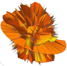
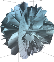
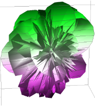
In order to account for the PGW effects on an even larger scale, with the possibility of each planet's resonant frequency being equal to the rate of acceleration, this would also imply the highly probable possibility of it also causing planetary accretion, and assembly of matter in a vacuum. Spherical Plots in 3D were simulated for each planet, again seeing if any observable anomalies appeared that coincided with real world observations.
Given the fact that each planet could have accreted and formed over an in-determinant amount of time, each resonant frequency for the spherical 3d plots was multiplied by the planet's radius in miles. This provides a to scale representation of each planet.
However our equation is still dependant on time, and a range of 0 to 1 does not provide the full sphere value. An arbitrary value of 10 was used as a control as it presented recognizable features compared to surrounding values that were either too much and became noise, or too little not plotting a full 360 degrees. This of course will require further validation and investigation, but has still provided some very impactful results. For the sake of saving computation, The author will highlight a few of the simulations here, but you can find the entire solar system, along with the sun, and even a black hole below.
In[16]:=
Grid[{{SphericalPlot3D[Sin[2 π g t]15759,{g,0,9.001},{t,0,6},MeshAutomatic,MeshFunctions{#3&}, ColorFunction"GreenPinkTones", PlotRange All, PlotLabel"Neptune X Radius", ImageSize->Large],
SphericalPlot3D[Sin[2 π g t]*t,{g,0,9.001},{t,0,6},MeshAutomatic,MeshFunctions{#3&}, ColorFunction"GreenPinkTones", PlotRange All, PlotLabel"Neptune X t"]}}]
SphericalPlot3D[Sin[2 π g t]*t,{g,0,9.001},{t,0,6},MeshAutomatic,MeshFunctions{#3&}, ColorFunction"GreenPinkTones", PlotRange All, PlotLabel"Neptune X t"]}}]
In[54]:=
Grid[{SphericalPlot3D[Sin[2 π g t]15299,{g,0,11.22287963},{t,0,10},MeshAutomatic,MeshFunctions{#3&}, ColorFunction"Aquamarine", PlotRange All, PlotLabel"Uranus X t"],
SphericalPlot3D[Sin[2 π g t]*t,{g,0,11.22287963},{t,0,10},MeshAutomatic,MeshFunctions{#3&}, ColorFunction"Aquamarine", PlotRange All, PlotLabel"Uranus X t"]}]
SphericalPlot3D[Sin[2 π g t]*t,{g,0,11.22287963},{t,0,10},MeshAutomatic,MeshFunctions{#3&}, ColorFunction"Aquamarine", PlotRange All, PlotLabel"Uranus X t"]}]
Our very own black hole at the center of the milky way was also simulated and can be found in the notebook here: https://www.wolframcloud.com/env/crkunferman/SagABlackHoleGR.nb
For a wider range of simulations and demonstrations you can view the notebook the author used here: https://www.wolframcloud.com/obj/crkunferman/gravity.nb:
For a wider range of simulations and demonstrations you can view the notebook the author used here: https://www.wolframcloud.com/obj/crkunferman/gravity.nb:
Experimental Result Analysis
Experimental Result Analysis
Discussion
Discussion
More
◼
Conclusion
The journey of discovery continues to surprise, and the charts and Data produced from this simple equation are showing nearly definitive evidence that the PGW is a fundamental aspect of our universe, but it doesn't end there.
◼
Future Work
In part 3 of this series, the author will showcase his work simulating the addition of Magnetic Fields to the PGW and will demonstrate the interplay of these forces on a cosmic scale, much larger than anything we have the ability to measure with our current technology.
Subsequent or additional studies, derived works and peer reviewed edits are most welcome! Simply copy your notebooks to the author so he may assess them, address any questions or corrections, and ultimately add them with credit to this amazing exploration.
The author looks forward to collaboration within the scientific community, for the greater understanding of humanity
◼
Supplemental
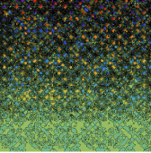
Further study was conducted of the PGW and while simulating earths PGW in Matlab, the author found what appears to be a double helix within a 3D Swarm Chart.
https://photos.app.goo.gl/w2Lq7hDy4WB8UYd46
The implications of this are immense, and warrant further study.
Additionally, this observation produced a unique way to search for life in the universe, under the assumption that a planet with a similar PGW and other habitable traits would have the same strand like structure that may have guided the evolution of life on our planet.
By searching exoplanet data, the list of candidates have been narrowed down to a list of 6. The Matlab code to conduct this survey is as follows:
% Constants
G = 6.67430e-11; % Gravitational constant in m^3 kg^-1 s^-2
earthMass = 5.972e24; % Earth's mass in kg
earthRadius = 6371e3; % Earth's radius in meters
% Define Earth-like Surface Gravity Range
minGravity = 9.8; % Lower bound (m/s^2)
maxGravity = 9.9; % Upper bound (m/s^2)
maxRadius = 1.5 * earthRadius; % Maximum radius (1.5 Earth radii)
% Fetch Exoplanet Data (mass, radius, and orbital data)
query = 'SELECT pl_name, pl_bmasse, pl_rade, pl_orbsmax, st_teff FROM pscomppars';
url = ['https://exoplanetarchive.ipac.caltech.edu/TAP/sync?query=', query, '&format=csv'];
filename = 'exoplanets.csv';
websave(filename, url);
% Load the data into MATLAB
data = readtable(filename);
% Convert mass and radius to SI units
data.MassKg = data.pl_bmasse * earthMass; % Convert mass to kg
data.RadiusM = data.pl_rade * earthRadius; % Convert radius to meters
% Calculate surface gravity
data.SurfaceGravity = (G * data.MassKg) ./ (data.RadiusM .^ 2); % in m/s^2
% Calculate PGW Frequencies
data.PGWFrequency = sin(2 * pi * data.SurfaceGravity);
% Filter for Earth-like planets
earthLikePlanets = data(data.SurfaceGravity >= minGravity & ...
data.SurfaceGravity <= maxGravity & ...
data.RadiusM <= maxRadius, :);
% Display refined Earth-like candidates
disp('Refined Earth-like Planets:');
disp(earthLikePlanets(:, {'pl_name', 'MassKg', 'RadiusM', 'SurfaceGravity', 'PGWFrequency', 'pl_orbsmax', 'st_teff'}));
% Visualize Surface Gravity vs Radius
figure;
scatter(data.SurfaceGravity, data.RadiusM / earthRadius, 'b', 'filled'); % All planets
hold on;
scatter(earthLikePlanets.SurfaceGravity, earthLikePlanets.RadiusM / earthRadius, 80, 'r', 'filled'); % Earth-like
xlabel('Surface Gravity (m/s^2)');
ylabel('Planet Radius (Earth Radii)');
legend('All Planets', 'Earth-like Planets');
title('Surface Gravity vs Radius (Refined)');
grid on;
hold off;
% Visualize PGW Frequencies
figure;
histogram(earthLikePlanets.PGWFrequency, 10);
xlabel('PGW Frequency');
ylabel('Number of Planets');
title('Distribution of PGW Frequencies for Earth-like Planets');
grid on;
% Visualize Habitable Zone Candidates (Semi-major axis vs Stellar Temp)
figure;
scatter(data.pl_orbsmax, data.st_teff, 'b', 'filled'); % All planets
hold on;
scatter(earthLikePlanets.pl_orbsmax, earthLikePlanets.st_teff, 80, 'r', 'filled'); % Earth-like
xlabel('Semi-Major Axis (AU)');
ylabel('Stellar Temperature (K)');
legend('All Planets', 'Earth-like Planets');
title('Habitable Zone Candidates');
grid on;
hold off;
% Save the refined dataset to a CSV file
writetable(earthLikePlanets, 'Refined_Earth_Like_Planets.csv');
disp('Refined Earth-like planets saved to Refined_Earth_Like_Planets.csv');
The code above produces the following results:
Refined Earth-like Planets:
pl_name MassKg RadiusM SurfaceGravity PGWFrequency pl_orbsmax st_teff
_________________ __________ __________ ______________ ____________ __________ _______
{'Kepler-197 b' } 6.2109e+24 6.4984e+06 9.8162 -0.91474 0.06 6004
{'Kepler-192 d' } 6.2109e+24 6.4984e+06 9.8162 -0.91474 0.0686 5487
{'Kepler-130 b' } 6.2109e+24 6.4984e+06 9.8162 -0.91474 0.079 5884
{'Kepler-1616 b'} 6.2109e+24 6.4984e+06 9.8162 -0.91474 0.07318 6266
{'Kepler-336 b' } 6.2109e+24 6.4984e+06 9.8162 -0.91474 0.033 5867
{'Kepler-1150 b'} 6.2109e+24 6.4984e+06 9.8162 -0.91474 0.0382 4754
Refined Earth-like planets saved to Refined_Earth_Like_Planets.csv