Perception & Analysis
Perception & Analysis
By: David Ameneyro. April 11, 2020.
This is my favorite picture from Stephen Wolfram’s A New Kind of Science:
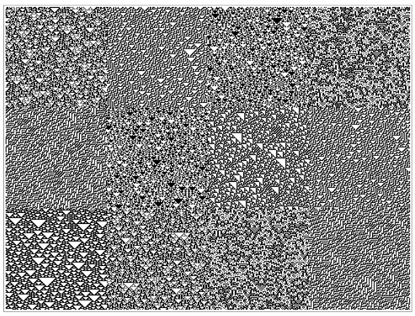
It's my favorite picture because it showed me how easily humans can process information when it’s encoded in a certain way, while—in contrast—having difficulty processing that same information encoded differently.
What are Cellular Automata?
What are Cellular Automata?
The picture above shows 12 patches with distinct textures. Although each patch looks "random", we can easily see where one patch ends and another begins. These patches are actually the outputs of simple programs called cellular automata. A cellular automaton is a simple program which generates data based on a set of rules like the following :
RulePlot[CellularAutomaton[30]]
Out[]=

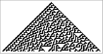
This rule is applied one row at a time, by looking at the cells in the prior row, and using those cells to determine the color of the cell in the current row. The rule above is Rule 30 of 256 possible rules that involve two colors (black or white), are two-dimensional, and use only the nearest neighbors to determine the color of the next cell. Rule 30 produces the following output after 50 steps, from a single initial black square:
ArrayPlot[CellularAutomaton[30,{{1},0},50]]
Out[]=
Different Ways of Encoding Cellular Automata
Different Ways of Encoding Cellular Automata
As you can see, that is similar to some of the patterns seen in the picture at the top. But that's the picture-form of a cellular automaton's output. Instead of black and white squares, the same information can be represented as 1s and 0s, with black squares being 1s and white squares being 0s.
CellularAutomaton[30,{{1},0},50]//Grid
Out[]=
Already we see that while the 1s and 0s above are the same exact data, it is much harder for us to identify any features in the data. And although the type-setting of the 1s and 0s do let us see a faint pyramid, this is again our visual processing system at work rather than any numerical or statistical analysis.
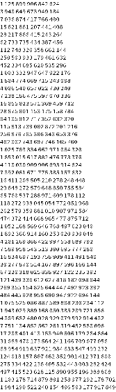
If we think about those 1s and 0s as binary digits with each row being a single integer, we can convert those binary digits to Base 10 and represent the same data like this:
FromDigits[#,2]&/@CellularAutomaton[30,{{1},0},50]//TableForm
Out[]//TableForm=
1125899906842624 |
3940649673949184 |
7036874417766400 |
15621861207441408 |
28217866415243264 |
62733735434387456 |
112748320358662144 |
250503933179461632 |
452334685620535296 |
1003332947647922176 |
1804774669715243008 |
4006540657022730240 |
7238186475597070336 |
16055023571369459712 |
28875001153175158784 |
64105912717352632320 |
115813739002872201216 |
256876765306343653376 |
462002743697746165760 |
1025703334662971064320 |
1853015617882476773376 |
4110030909906693914624 |
7392061671775385157632 |
16411208505210278248448 |
29648272579648850755584 |
65760537288971609178112 |
118272938045054772051968 |
262579359881010907971584 |
474372414668965477875712 |
1052168569646768497623040 |
1892366914160253020930048 |
4201269868422997558689792 |
7589958543513300695777280 |
16834697193758909411491840 |
30277870514167897596166144 |
67220318025838927122235392 |
121439336612627818182098944 |
269355154825644447492923392 |
484445928958690947922694144 |
1075525086887589808230234112 |
1943029389168050385209721856 |
4309682480028929079592914432 |
7751134852562261319452580096 |
17208401413153940606179284864 |
31088470173564241166709077056 |
68954919637921984633547499232 |
124018157807462352901412371600 |
275334422236405532443003282424 |
497415523628125890955196388868 |
1103278714879801258977292178702 |
1984290522240154406503177917849 |
Again, this is the same data as the 1s and 0s and the pyramid picture above, but in Base 10 numeric form. In this form the only distinguishing feature we can readily identify is that the numbers are getting progressively larger. This is mostly a consequence of the initial conditions we chose (starting from a single bit of data), and if we applied that same rule to random initial conditions, we would see more or less uniformly large numbers in each row.
In[]:=
FromDigits[#,2]&/@CellularAutomaton[30,RandomInteger[1,100],10]//TableForm
Out[]//TableForm=
335890346574594295376971296202 |
1139324344492791762802066852155 |
144629273005651540768112779234 |
247083640597804249176622510103 |
1164225457868663479480231684148 |
686778231555374161601340689511 |
448974754395931858298148207324 |
1043163832215612110405693481618 |
785704601674538028671735396094 |
1191711252860082419249065903232 |
681699722093922735540121890753 |
So now we' ve seen three very different ways to represent the same exact data :
Rasterize[#,RasterSize1000]&/@{ArrayPlot[CellularAutomaton[30,{{1},0},50]],CellularAutomaton[30,{{1},0},50]//Grid,FromDigits[#,2]&/@CellularAutomaton[30,{{1},0},50]//TableForm}
Out[]=
,

,
Although the three pictures above show the same exact data, we process each encoding of the data differently.
Next I want to demonstrate that while we can easily identify differences in the visually-encoded data (see the very top picture). We cannot readily identify differences in either the Base 2 or Base 10 encodings.
Next I want to demonstrate that while we can easily identify differences in the visually-encoded data (see the very top picture). We cannot readily identify differences in either the Base 2 or Base 10 encodings.
Perceiving Data
Perceiving Data
The following picture is like the picture at the beginning of this post, except that it shows only two different textures, made from two different cellular automata rules:
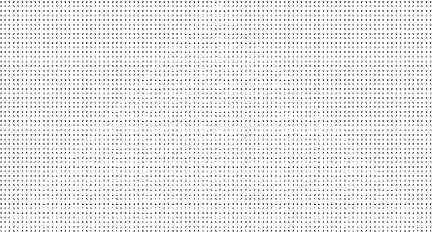
The line between the two textures is still readily identifiable. Now let’s look at that same data but encoded as 1s and 0s:
The same data appears similar without any clear indication where the output of one program ends and the other begins. Now let’s encode in Base 10 to see if we can tell the difference.
Again after close scrutiny, we can’t tell where the output of one program begins and the other ends, even though it is the same data as the picture.
Even when viewing the three different encodings side by side we can’t see distinctions in the two outputs in numeric form like we can when plotted as an array.
Even when viewing the three different encodings side by side we can’t see distinctions in the two outputs in numeric form like we can when plotted as an array.
Criticisms
Criticisms
A fair criticism of my approach above is that the first encoding is visual, while the other two are numeric. However, we do have another way of visualizing this data that we haven’t explored—we can plot the data in a Line Chart.
The plot above is the same data as the prior encodings, but we still can’t identify where one output ends and the second output begins.
After finishing & publishing this post I realized that the way I coded all of the above, I didn’t actually use the exact same data between comparisons. I used RandomInteger to generate random initial conditions, but since I called that function each time I plotted the data, I got new random initial conditions. I should have saved a random initial condition and used that in all the plots so I would have the exact same data.
That said, the specific cellular automata I used tend to output very similar patterns regardless of the initial conditions.
That said, the specific cellular automata I used tend to output very similar patterns regardless of the initial conditions.
Each of the plots above are generated using Rules 30 & 45, with random initial conditions for every instance. As we can see, the outputs between the same programs is different, but still similar enough that my larger point remains valid.
I will update this post using the same initial conditions between comparisons if I find the time.
I will update this post using the same initial conditions between comparisons if I find the time.
Next Up
Next Up
In the next post we’ll explore different statistical/programmatic analyses of this data to see if there are other rules-based ways that we can distinguish the output of two different cellular automata.
Bibliography
Bibliography