1. Using FluidFlowPDEComponent for the Navier-Stokes part
1. Using FluidFlowPDEComponent for the Navier-Stokes part
Fluid Dynamics Model
Fluid Dynamics Model
Use of FluidFlowPDEComponent for the Navier-Stokes part was achieved by first comparing the coefficients in the Brinkman momentum equation with the coefficients in the Navier-Stokes momentum equation:
Navier-StokesEquation:0V+
ρV·∇V+∇·(-μ∇V)+∇p | = | 0 |
BrinkmanEquation:
μ κ μ ϕ | = | F |
Thus, FluidFlowPDEComponent can be used to solve the Navier-Stokes part by modifying it in the following way:
1
.Making the following replacements in the function parameters for region 2:
1
.1
.Replacing the mass density ρ with 0.
1
.2
.Replacing the dynamic viscosity μ with .
μ
ϕ
2
.Adding the term V to the function for region 2.
μ
κ
3
.Defining the continuity equation explicitly in its reduced form . This adjustment is necessary because we replaced ρ with 0, which would otherwise cause the continuity equation to become an identity in region 2.
∇·V=0
Making the aforementioned modifications in the FluidFlowPDEComponent gives the following flow model:
In[]:=
coupledFlowModel=FluidFlowPDEComponent{{u[x,y],v[x,y],p[x,y]},{x,y}},<|"DynamicViscosity"->IfElementMarker==1,μ,,"MassDensity"->If[ElementMarker==1,ρ,0]|>+IfElementMarker==1,0,*{u[x,y],v[x,y],0};coupledFlowModel[[-1]]=[x,y]+[x,y];
μ
ϕ
μ
κ
(0,1)
v
(1,0)
u
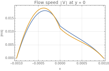
This model reproduces the result of the original notebook provided as shown below.
Model Implementation
Model Implementation
In[]:=
Needs["NDSolve`FEM`"];
In[]:=
coordinates=;
In[]:=
connectivity=;
In[]:=
bmesh=ToBoundaryMesh["Coordinates"coordinates,"BoundaryElements"connectivity];
In[]:=
freeCoordinate={-5*,0};
-4
10
In[]:=
porousCoordinate={5*,0};
-4
10
In[]:=
mesh=ToElementMesh[bmesh,"RegionMarker"->{{freeCoordinate,1},{porousCoordinate,2}},"MaxCellMeasure"{"Length"2*}];
-4
10
In[]:=
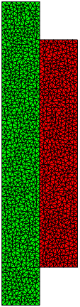
mesh["Wireframe"["MeshElementStyle"{Directive[FaceForm[Green]],Directive[FaceForm[Red]]}]]
Out[]=
In[]:=
μ=(*dynamicviscosity*);ρ=1000(*pristinewaterdensity*);κ=(*permeability*);ϕ=0.4(*porosity*);=0.02(*inletvelocity*);=0(*referencepressure*);Cf=(*frictioncoefficient*);
-3
10
-7
10
v
in
p
ref
1.75
150
3
ϕ
In[]:=
{,}=IfElementMarker1,0,-*+*{u[x,y],v[x,y]};
F
x
F
y
ρϕCf
κ
2
u[x,y]
2
v[x,y]
In[]:=
Γ
inlet
v
in
-3
10
In[]:=
Γ
outlet
p
ref
-3
10
In[]:=
Γ
wall
-3
10
-3
10
-3
10
In[]:=
bcs={,,};
Γ
inlet
Γ
outlet
Γ
wall
In[]:=
pde={coupledFlowModel{0,0,0},bcs};
In[]:=
{ufun,vfun,pfun}=NDSolveValue[pde,{u,v,p},{x,y}∈mesh,"InitialSeeding"{u[x,y]0,v[x,y],p[x,y]0},Method{"PDEDiscretization"{"FiniteElement","InterpolationOrder"{u2,v2,p1}}}];
v
in
In[]:=
pde={coupledFlowModel{,,0},bcs};
F
x
F
y
In[]:=
{ufunCorrected,vfunCorrected,pfunCorrected}=NDSolveValue[pde,{u,v,p},{x,y}∈mesh,"InitialSeeding"{u[x,y]ufun[x,y],v[x,y]vfun[x,y],p[x,y]0},Method{"PDEDiscretization"{"FiniteElement","InterpolationOrder"{u2,v2,p1}}}];
In[]:=
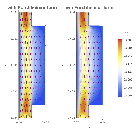
g1=;g2=;lis=&/@{g1,g2};GraphicsRow[lis]
Out[]=
In[]:=
Plot+,+,x,-,,PlotTheme"Detailed",PlotLegends{"with correction","w/o correction"},PlotLabelStyle["Flow speed V at y = 0",14],FrameLabel{"x","[m/s]"},ImageSizeMedium
2
ufun[x,0]
2
vfun[x,0]
2
ufunCorrected[x,0]
2
vfunCorrected[x,0]
1
3
10
1
3
10
Out[]=