Effect of window on spectral line width and SFDR
Effect of window on spectral line width and SFDR
In[]:=
f_samp=1000;(*samplingfrequency[Hz]*)
In[]:=
T_samp=1/f_samp;(*samplingperiod[s]*)
In[]:=
N_s=1024;(*numberofthepointsofDFT*)
When the tone frequency is an integer multiple of sampling frequency divided by the number of the points of DFT
When the tone frequency is an integer multiple of sampling frequency divided by the number of the points of DFT
In[]:=
f_tone=f_samp*8/N_s;(*tonefrequency[Hz]*)
In[]:=
A_tone=1;(*toneamplitude*)
In[]:=
x_s=Table[A_tone*Sin[2Pi*f_tone*T_samp*n],{n,0,N_s-1}];(*tonesignal*)
In[]:=
A_noise=1/8;(*noiseamplitude*)
In[]:=
x_n=RandomReal[{-A_noise/2,A_noise/2},N_s];(*randomnoise*)
In[]:=
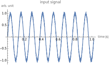
x_in=x_s+x_n;
In[]:=
ListLinePlot[x_in,DataRange{0,(N_s-1)*T_samp},PlotLabel"input signal",AxesLabel{"time [s]","arb. unit"}]
Out[]=
In[]:=
X_in=Fourier[x_in,FourierParameters{0,-1}];(*DFTofinputsignal*)
In[]:=
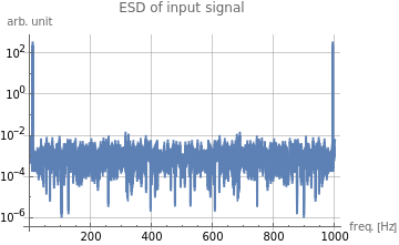
ESD_X_in=(Re[#]^2+Im[#]^2)&/@X_in;
In[]:=
ListPlot[ESD_X_in,DataRange{0,f_samp*(N_s-1)/N_s},ScalingFunctions"Log10",JoinedTrue,PlotLabel"ESD of input signal",AxesLabel{"freq. [Hz]","arb. unit"},GridLinesAutomatic]
Out[]=
In[]:=
ESD_X_in[[N_s-8;;N_s]]
Out[]=
{0.000273698,255.779,0.0059571,0.00026995,0.000935302,0.00209327,0.000894437,0.00426643,0.00628362}
In[]:=
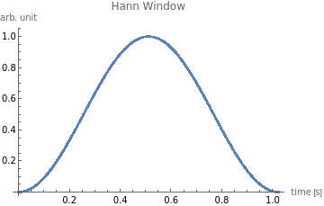
w_Hann=Table[Sin[Pi*n/N_s]^2,{n,0,N_s-1}];
In[]:=
ListPlot[w_Hann,DataRange{0,(N_s-1)*T_samp},PlotLabel"Hann Window",AxesLabel{"time [s]","arb. unit"}]
Out[]=
In[]:=
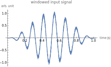
wnd_x_in=w_Hann*x_in;
In[]:=
ListLinePlot[wnd_x_in,DataRange{0,(N_s-1)*T_samp},PlotLabel"windowed input signal",AxesLabel{"time [s]","arb. unit"}]
Out[]=
In[]:=
wnd_X_in=Fourier[wnd_x_in,FourierParameters{0,-1}];(*DFTofwindowedinputsignal*)
In[]:=
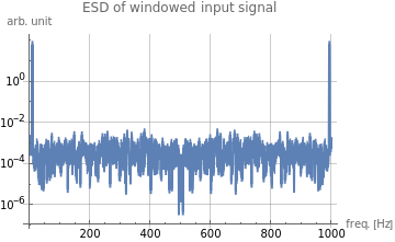
ListPlot[(Re[#]^2+Im[#]^2)&/@wnd_X_in,DataRange{0,f_samp*(N_s-1)/N_s},ScalingFunctions"Log10",JoinedTrue,PlotLabel"ESD of windowed input signal",AxesLabel{"freq. [Hz]","arb. unit"},GridLinesAutomatic]
Out[]=
When the tone frequency is not an integer multiple of sampling frequency divided by the number of the points of DFT
When the tone frequency is not an integer multiple of sampling frequency divided by the number of the points of DFT
In[]:=
f_tone_2=f_samp*7.5/N_s;
In[]:=
x_s_2=Table[A_tone*Sin[2Pi*f_tone_2*T_samp*n],{n,0,N_s-1}];
In[]:=
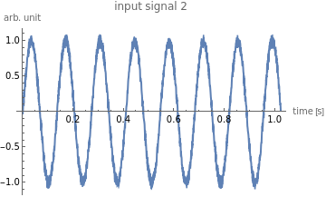
x_in_2=x_s_2+x_n;
ListLinePlot[x_in_2,DataRange{0,(N_s-1)*T_samp},PlotLabel"input signal 2",AxesLabel{"time [s]","arb. unit"}]
Out[]=
In[]:=
X_in_2=Fourier[x_in_2,FourierParameters{0,-1}];
In[]:=
pow_X_in_2=(Re[#]^2+Im[#]^2)&/@X_in_2;
ListPlot[pow_X_in_2,DataRange{0,f_samp*(N_s-1)/N_s},ScalingFunctions"Log10",JoinedTrue,PlotLabel"power frequency spectrum of input signal 2",AxesLabel{"freq. [Hz]","arb. unit"},GridLinesAutomatic]
Out[]=
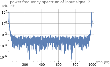
pow_X_in_2[[N_s-8;;N_s]]
Out[]=
{9.45557,96.8788,111.145,14.3192,6.03801,3.47421,2.62603,2.28979,1.92439}
Note that the peak is composed of two different height spikes at (0 based) index N_s-8 and N_s-7.
In[]:=
wnd_x_in_2=w_Hann*x_in_2;
In[]:=
wnd_X_in_2=Fourier[wnd_x_in_2,FourierParameters{0,-1}];
In[]:=
pow_wnd_X_in_2=(Re[#]^2+Im[#]^2)&/@wnd_X_in_2;
Note that the peak is composed of two adjacent nearly equal height spikes.