Wolfram Knowledgebase | Things to Try
Wolfram Knowledgebase | Things to Try
Make edits and run any piece of code by clicking inside the code and pressing .
+
Instant Access to Real-World Data. Compute with and visualize a growing collection of carefully curated data across hundreds of essential domains, seamlessly integrated with the entire Wolfram Language.
Compute with Geographic Data
Compute with Geographic Data
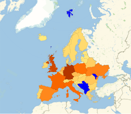
Create a map with geographic data (this may take longer to evaluate): |
In[]:=
GeoRegionValuePlot->"GreenhouseGasEmissions",MissingStyle->Blue
Out[]=
Retrieve a collection of data for each country: |
In[]:=
rawdata=EntityValueEntityClass["Country","Countries"],,,,;
Delete missing data and group by continent: |
In[]:=
cleandata=GroupBy[DeleteMissing[rawdata,1,1],Last,MapApply[Function[{pov,gdp,pop},{pov,QuantityMagnitude[gdp],pop}]]];
Plot the cleaned data: |
In[]:=
BubbleChartcleandata,
Compute with Physical Quantities
Compute with Physical Quantities
Retrieve wavelengths for a class of spectral lines: |
In[]:=
wavelengths=EntityValue,;
Plot these lines in the visible spectrum: |
In[]:=
GraphicsMap[{ColorData["VisibleSpectrum"][#],Line[{{#,0},{#,1}}]}&,QuantityMagnitude[wavelengths,"Nanometers"]],
Retrieve thermodynamic data for substances: |
In[]:=
substances={"Water","Methanol","Octane"};temps=Quantity[Range[1,130],"DegreesCelsius"];densitydata=Table[{temps,ThermodynamicData[substance,"Density",{"Temperature"->temps}]}//Transpose,{substance,substances}];
Visualize the retrieved data: |
In[]:=
ListLinePlot[densitydata,AxesLabel->Automatic,PlotLegends->substances]
Compare the sharp density decreases in the plot with known boiling points: |
In[]:=
EntityValue[Interpreter["Chemical"][substances],"BoilingPoint","Association"]
Compute with Biological and Ecological Data
Compute with Biological and Ecological Data
Plot the location of anatomical structures in 3D: |
In[]:=
AnatomyPlot3D,
Compare anatomical entities: |
In[]:=
organs=,,;properties={"Mass","CellCount"};ListPlot[EntityValue[organs,properties,"Association"],AxesLabel->properties]
Define biosequences and explore their structural properties: |
In[]:=
insulin=;MoleculePlot[Molecule[insulin]]
Define a class of entities for data retrieval: |
In[]:=
endangeredMammal=EntityClass"TaxonomicSpecies",->,->;
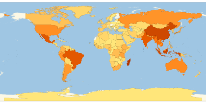
Visualize the number of endangered mammals present by country: |
In[]:=
GeoRegionValuePlot[EntityValue[endangeredMammal,"ObservationCountries"]//Flatten//Tally]
Out[]=
Analyze Financial Data
Analyze Financial Data
Retrieve financial data and present it in a standard format: |
In[]:=
TradingChart["GE",{"Volume","SimpleMovingAverage","BollingerBands"}]
Interpret financial entities from text: |
In[]:=
stocks=Interpreter["Financial"][{"GOOGL","MSFT","AAPL"}]
Compare properties of entities over time: |
In[]:=
property=;DateListPlotEntityValuestocks,Datedproperty,Interval,Yesterday,PlotLegendsCommonName[stocks]
Compute with Socio-Cultural Data
Compute with Socio-Cultural Data
Visualize the genre preferences of an artist: |
In[]:=
genres=EntityValueEntityClass"Artwork","Artist"->,"ArtGenre"//Flatten;PieChart[Counts[genres],ChartLabels->Automatic]
Retrieve construction start dates from an implicitly defined class of castles: |
In[]:=
castleAndYear=EntityValueEntityClass"Castle",->,"ConstructionStartDate","NonMissingEntityAssociation";
Look for trends in time: |
In[]:=
DateHistogram[castleAndYear,{{900},{1300},"Decade"}]
Organize the data from a particularly active period: |
In[]:=
castlesOfInterest=SelectcastleAndYear,≤#≤&;castlesByDecade=GroupBy[castlesOfInterest//Normal,DateObject[#[[2]],"Decade"]&,Map[First]]//KeySort


