Wolfram Visualization | Things to Try
Wolfram Visualization | Things to Try
Make edits and run any piece of code by clicking inside the code and pressing .
+
Scientific, Data & Function Visualization. Wolfram visualizations simplify and automate the creation of plots used to understand data and functions for everything from personal explorations to reports and published papers.
Explore Data Visually
Explore Data Visually
Visualize trends in data with dozens of available plot types: |
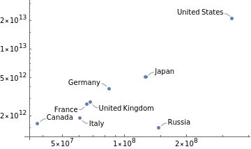
ListPlot[{"Population","GDP"}]["Name"],ScalingFunctions{"Log","Log"}
Out[]=
Easily visualize proportions with a pie chart: |
PieChart["Population"],ChartLabels->["Name"]
Easily compare data across categories with a bar chart: |
BarChart["Population"],ChartLabels->["CountryCode"]
Label and visualize data across multiple levels of organization: |
BarChart,,ChartLabels->["CountryCode"],None,ChartLegends->{"2005","2020"}
Style Your Plots
Style Your Plots
Define and plot a set of functions: |
functions=Table[BesselJ[n,x],{n,4}];Plot[Evaluate[functions],{x,0,10}]
Use |
Plot[Evaluate[functions],{x,0,10},PlotTheme->"Detailed"]
Create a list showing different themes to easily compare: |
Table[Plot[Evaluate[functions],{x,0,10},PlotTheme->theme,PlotLabel->theme],{theme,{"Minimal","Marketing","Monochrome"}}]
Set options individually or combine options with an overall theme: |
Plot[Evaluate[functions],{x,0,10},PlotTheme->"Marketing",PlotLegends->"Expressions"]
Label Your Plots
Label Your Plots
Use the |
countrydata=,;countrynames=["Name"];
Visualize the data retrieved: |
ListLogLogPlot[countrydata]
Use metadata to automatically label each data point (labels that do not fit are automatically generated as a tooltip): |
ListLogLogPlot[countrydata->countrynames]
Include labels for the frame and overall title to complete the visualization: |
ListLogLogPlot[countrydata->countrynames,Frame->True,PlotLabel->"Per capita GDP vs. Population for all Countries",FrameLabel->{"People","USD per person per year"}]
Plot Functions
Plot Functions
Plot a function of a single variable over a specified domain: |
Plot[Tan[x],{x,-3Pi/2,3Pi/2}]
Plot a parametric function over a specified parameter range: |
ParametricPlot[{Cos[Pit]*GoldenRatio^t,Sin[Pit]*GoldenRatio^t},{t,0,6}]
Use the 3D versions of plotting functions: |
ParametricPlot3D{Cos[πt](+Cos[v]),(+Cos[v])Sin[πt],4t-Sin[v]},{t,0,5},{v,0,2Pi},
t
GoldenRatio
t
GoldenRatio
Use options to make a stylized 3D plot of a function: |
Plot3DTan+,{x,y}∈Disk[{0,0},10,{Pi/2,3Pi/2}],
2
x
2
y
Make Visualizations Interactive
Make Visualizations Interactive
Easily create interactive displays: |
ManipulateParametricPlot3D,{t,0,tmax},{v,0,vmax},,{{vmax,2Pi,"Maximum v parameter"},Pi/2,2Pi},{{tmax,3,"Maximum t parameter"},1,5},ControlPlacement->Top,SaveDefinitions->True,TrackedSymbols:>{vmax,tmax}
Out[]=
Visualize Vector Fields
Visualize Vector Fields
Visualize electric field lines for a dipole: |
In[]:=
StreamPlot3D-,{x,-3,3},{y,-3,3},{z,-3,3}
{x,y,z-1}
3
Norm[{x,y,z-1}]
{x,y,z+1}
3
Norm[{x,y,z+1}]
Bound the magnitude of the vector field norm with a region function to make the rapid change near the point charges at z=±1 |
Plot Complex Functions
Plot Complex Functions
Visualize Volumetric Data
Visualize Volumetric Data
Create Geography Graphics
Create Geography Graphics


