2.3 Law of Large Numbers
2.3 Law of Large Numbers
The Law of Large Numbers tells us that as the sample average defined by
n→∞
x
1
n
n
∑
i=1
X
i
will be near the population average μ with a given probability. Given samples from a population, we don’t expect X to exactly match μ. The Law of Large Numbers allows us to make a statement about the difference -μ. Specifically, the statement involves the probability that is smaller than a certain value.
n
X
-μ
X
To answer the following questions, you do not need to understand the Law of Large Numbers. However, if you are interested, more formal definitions and proofs are given in
◼
Orloff and Bloom, Reading 6b
◼
Bulmer, Chapter 6
◼
DeGroot, Chapter 6
◼
Rozanov, p 69
Assigned tasks part a
Assigned tasks part a
1
.Draw values from a population of Gaussian-distributed number with mean and standard deviation .
n=100
μ=0
σ=1
In[]:=
take[n_]:=RandomVariate[NormalDistribution[],n]
2
.Compute .
X
In[]:=
x
Out[]=
-0.140964
3
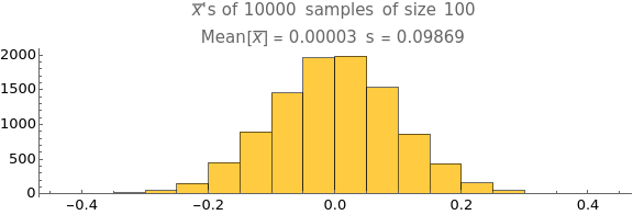
.Repeat 1 and 2 10000 times and plot a histogram of .
X
In[]:=
Histogram[tbl100=Table[Mean[take[100]],{10000}],PlotLabel->Column[{"'s of 10000 samples of size 100",Row[{"Mean[] = ",Round[Mean[tbl100],.00001]," s = ",Round[StandardDeviation[tbl100],.00001]}]},Center],LabelStyle->13,AspectRatio->1/4,PlotRange->All,ImageSize->Large]
x
x
Out[]=
Assigned tasks part b
Assigned tasks part b
1
.For , what fraction of the 10000 s were in the range [-0.01,0.01]?
n=100
X
In[]:=
exact=,N[exact]
Count[Table[Mean[take[100]],{10000}],x_/;x<=.01]
10000
Out[]=
,0.0738
369
5000
2
.How does the fraction depend on ?
n
The fraction approaches 1 as . Since the samples are taken without replacement, there is no guarantee the fraction will reach 1 in finite . But the Law of Large Numbers holds that it will become arbitrarily close. By that, I mean for any real error , no matter how small, the Law guarantees there will be some beyond which all ±1 will be less than ϵ for all .
n->∞
n
ϵ>0
N∈
X
n
n>N
In[]:=
tbl=Table,,{n,1,6};
n
10
CountTable[Mean[take[]],{10000}],x_/;x<=
n
10
1
100
10000
In[]:=
ListLogLogPlotTable[Labeled[tbl[[i]],N[tbl[[i,2]]]],{i,1,Length[tbl]}],AspectRatio->,Joined->True,PlotMarkers->Automatic,ImageSize->Large,LabelStyle->12,PlotRange->{0,1},PlotLabel->"Fraction of 10000 samples with ∈ 0 ± 0.01",AxesLabel->{"Sample Size",""},ImagePadding->Automatic
1
3
X
Out[]=

3
.For , what is the range for which 99% of the 10000 s fall in?
n=100
[-ϵ,ϵ]
X
In[]:=
Sort[(tbl100-Mean[tbl100])][[{51,-51}]]
Out[]=
{-0.258892,0.252217}
4
.How does ϵ depend on ?
n
Itfollowsfromthanswertoprompt2abovethatϵ=0.
lim
n->∞
5
.How does your answer change if the distribution changes (that is, if you draw values from a distribution other than Gaussian)?
Answer may be different. One assumption needed for CLT to apply is a finite mean and standard deviation. PDF for , for example, has no finite mean or variance, xx=∞. I assume other assumptions protect the theorem from distributions like mean weight of samples from an urn with 5 million objects of weight 1 and one of weight 5 million, even though that would have finite μ, σ.
1
2
x
x>=1
∞
∫
1
1
2
x
590 students: Be prepared to discuss in class how this experiment is related to the Law of Large Numbers.
2.4 Central Limit Theorem
2.4 Central Limit Theorem
The Central limit Theorem says that for large n, = is Gaussian-distributed with mean μ and standard deviation . Important : this theorem (usually) applies even if the distribution of the values used in computing X are not Gaussian—distributed. With the Central Limit Theorem, we can make statements such as, “I took a sample of values and computed . If I took many samples and computed many s, 95% of the time the range ±1.96 would include μ.”
X
1
n
n
∑
i=1
X
i
σ
n
n
X
X
X
σ
n
Verify CLT
Verify CLT
In the previous problem, you computed a histogram of 10000 s. Based on Central Limit Theorem,... Create one or two plots that demonstrate these points. Pay attention to your annotations. Save y our code as HW2_4. and plots as HW2_4.png (use subplots).
X
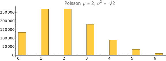
Take a large Poisson distribution , which is heavily skewed.
μ=2
In[]:=
poisson=RandomVariate[PoissonDistribution[2],{1000000}];Histogrampoisson,,PlotLabel->"Poisson μ = 2, =
1
3
2
σ
2
",AspectRatio->13,LabelStyle->13,ImageSize->LargeOut[]=
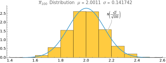
Then show distribution of is normal with mean and standard deviation ≈2ands≈.
x
100
x
2
100
In[]:=
means100=Table[Mean[RandomSample[poisson,100]],{10000}];ShowHistogram[means100,Automatic,"PDF",LabelStyle->13,PlotLabel->Row[{Distribution," μ = ",N[Mean[means100]]," σ = ",N[StandardDeviation[means100]]}]],PlotCalloutPDFNormalDistribution2,,x,Row,{2.2,2},{x,3/2,5/2},ImageSize->Large,AspectRatio->13
x
100
2
100
N
2
100
Out[]=
Except when it doesn’t
Except when it doesn’t