What Is Quantum Computation?
What Is Quantum Computation?
In[]:=
<<Wolfram`QuantumFramework`
Key Concepts
Key Concepts
◼
Quantum Circuit
◼
Qubit
◼
Measurement
Classical Computation
Classical Computation
In order to understand quantum computation, it helps to compare it to classical computation. To compute something, you have to be able to use rules to determine what should be the output from a list of inputs. You can think of computing as starting with the inputs and following the rules to reach an output.
Below is the definition of a simple function that accepts two binary strings as input and returns their sum also as a binary string:
In[]:=
fadder[str1_String,str2_String]/;:=IntegerString[FromDigits[str1,2]+FromDigits[str2,2],2]
In[]:=
fadder["01","01"]
Out[]=
10
In[]:=
fadder["100","011"]
Out[]=
111
This function is explicitly defined in terms of other Wolfram Language™ functions. However, it is implicitly defined as a bunch of rules that tell you how to go from two binary strings of given lengths to some other binary string of a needed length:
fadder:↦
a
{0,1}
b
{0,1}
c
{0,1}
Classical Bits and Encodings
Classical Bits and Encodings
You may already be familiar with the fact that classical computations can be represented by operations on sequences of bits. A classical bit has a state which is either a 0 or a 1. What are all the states of a sequence of four classical bits?
In[]:=
fourbits=Tuples[{"0","1"},4]//Map[StringJoin]
Out[]=
{0000,0001,0010,0011,0100,0101,0110,0111,1000,1001,1010,1011,1100,1101,1110,1111}
It is also possible to encode information in such sequences of classical bits to represent problems of interest. For example, each of those bit sequences can encode an integer in the base 2 number system. (This is utilized by the example function ):
fadder
In[]:=
Map[s|->FromDigits[s,2],fourbits]
Out[]=
{0,1,2,3,4,5,6,7,8,9,10,11,12,13,14,15}
Each of those bit sequences could also encode letter characters with a different encoding scheme:
In[]:=
Map[s|->FromLetterNumber[FromDigits[s,2]],fourbits]
Out[]=
{ ,a,b,c,d,e,f,g,h,i,j,k,l,m,n,o}
With yet another encoding scheme, those same bit sequences could represent colors with opacity:
In[]:=
Map[s|->Apply[RGBColor,FromDigits/@Characters[s]],fourbits]
Out[]=
,,,,,,,,,,,,,,,
As you can see, a lot of classical computing can be thought of as representing a problem of interest as a sequence of bits, using some rules to compute another sequence of bits, then decoding the result to get your solution. Let’s see one more example before moving on to quantum computation.
The usual Plus function doesn’t have rules for adding colors:
In[]:=
Red+Blue
Out[]=
Let’s define a function that encodes the colors as sequences of zeros and ones, performs a computation on those sequences, then decodes the result as another color. For illustration purposes this function uses to show the intermediate bit sequences:
In[]:=
fblender[col1_,col2_]:=RGBColor@@Echo@MapThread[BitOr,Echo@MapApply[List,{col1,col2}]]
In[]:=
fblender[Red,Blue]
»
{{1,0,0},{0,0,1}}
»
{1,0,1}
Out[]=
Note that the last example function differs from the built-in function, because it follows different rules to transform the intermediate bit strings:
fblender
In[]:=
Blend[{Red,Blue}]
Out[]=
In[]:=
List@@%
Out[]=
,0,
1
2
1
2
Quantum Circuits and Qubits
Quantum Circuits and Qubits
The diagram below represents an example of a quantum circuit:
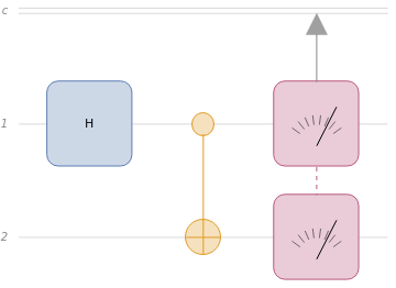
Notice how the circuit diagram has several wires, labeled , 1 and 2. Wires 1 and 2 represent qubits (quantum bits) instead of classical bits. The boxes that look like gauges on the right hand side of the diagram represent measurement and point to the wire labeled . The wire labeled represents a classical system (such as part of a regular computer) where the results of the measurements on qubits are stored.
c
c
c
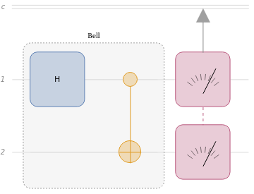
To create a circuit diagram like the one seen above, you first specify a circuit and then use the property of that circuit.
"Diagram"
In[]:=
examplecircuit=QuantumCircuitOperator[{"Bell","M"->{1,2}}];examplecircuit["Diagram"]
Out[]=
What are the results of running this circuit?
In[]:=
measurements=examplecircuit[]
Out[]=
QuantumMeasurement

Since the last operation in the circuit is a measurement, the result of evaluating the circuit is a object. What are the results of the measurement in this circuit?
In[]:=
measurements["ProbabilitiesPlot"]
Out[]=
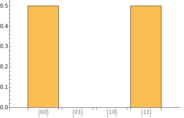
Notice that the possible outcomes of the measurement are just classical bit sequences. In the previous examples of classical computation, the rules for computing were deterministic. You got a definite result for any given inputs. In quantum computation, the rules of computation will generally give you probabilities of measuring several possible outcomes. For a quantum program to be useful, you want to arrange things so that the probability of measuring a result that encodes the solution to your problem is high.
In[]:=
measurements["Probabilities"]
Out[]=
00,010,100,11
1
2
1
2
In this example, the probability of obtaining “00” is 1/2, the probability of obtaining “11” is 1/2, and the probability of obtaining the “01” or “10” measurement outcomes is zero. While qubits are not the same as classical bits (otherwise quantum algorithms would be no different from classical ones), you will always perform some kind of measurement as part of a practical quantum circuit.
The other symbols in the quantum circuit represent instructions for what operations to perform on the qubits. The next lessons will discuss them in much greater detail.
Example
Example
Consider the quantum circuit below. What are the probabilities of measuring each of the 6-bit classical outcomes?
In[]:=
explorecircuit=QuantumCircuitOperator;explorecircuit["Diagram"]
Out[]=
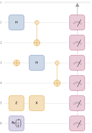
Solution
Example
Example
Consider the quantum circuit below. What are the probabilities of measuring each of the 4-bit classical outcomes? Plot the probability distribution.
Solution
The non-zero probability outcomes are shown:
The entire distribution is shown: