Building Blocks of Quantum Circuits
Building Blocks of Quantum Circuits
In[]:=
<<Wolfram`QuantumFramework`
Key Concepts
Key Concepts
◼
Quantum Operator
◼
Quantum State
◼
Register State
◼
Bloch Sphere
◼
Computational Basis
Quantum Operations
Quantum Operations
In the last lesson, you saw the following quantum circuit:
In[]:=
QuantumCircuitOperator[{"Bell","M"->{1,2}}]["Diagram"]
Out[]=
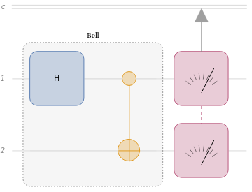
The symbols inside the gray box represent quantum operators. Remember that classical computation involves rules that tell you how to go from input states to output states. Quantum operators are just the rules that transform one quantum state into another. They follow special constraints that come from the formalism of quantum mechanics. You will often hear quantum operators referred to as “gates” or “gate operations” as well. This terminology comes from classical computer engineering.
Quantum States
Quantum States
Recall that states in classical digital computing can be represented by sequences of 1s and 0s. Each classical bit has two possible states, 0 or 1. A sequence of two classical bits has four possible states: “00”, “01”, “10” or “11”. A sequence of classical bits has possible states.
n
n
2
When quantum states are measured, you always get a particular classical result after performing the measurement. However, interacting with the system to measure it always involves changing its state in some way. In general, a quantum state is not the same as a classical state. However, some quantum states will always give the same classical state when measured. Such qubit states can simply be labeled by a classical bit sequence.
For example, if quantum operators in a circuit diagram represent instructions for changing the quantum state, you may have wondered what is the input state? By convention, most quantum circuit diagrams begin with the register state. The register state is just the quantum state that always gives the result of all zeros when the qubits are measured.
The 1-qubit register state can be written as follows:
In[]:=
QuantumState["Register"]["Formula"]
Out[]=
|0〉
The 2-qubit register state can be written like this:
In[]:=
QuantumState["Register"[2]]["Formula"]
Out[]=
|00〉
And so on:
In[]:=
Table[QuantumState["Register"[n]]["Formula"],{n,3,6}]
Out[]=
{|000〉,|0000〉,|00000〉,|000000〉}
While some quantum states always give the same result for the same measurements, it is important to remember that this is not the case for all quantum states. Future examples will examine this in more detail.
The Bloch Sphere
The Bloch Sphere
Since qubits are not the same as classical bits, labeling them by classical bit sequences is insufficient to represent all possible qubit states. How then are quantum states represented?
Future lessons will discuss representing quantum states with matrices. In fact, much of the formalism of quantum mechanics is an important application of linear algebra. However, there is a very useful graphical representation of 1-qubit states called the Bloch sphere.
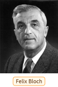
The Bloch sphere is named after physicist Felix Bloch:
The Bloch sphere representation of the qubit state can be given as follows:
|0〉
In[]:=
QuantumState["0"]["BlochPlot"]
Out[]=

Notice that the qubit state is on the opposite side of the sphere from .
|1〉
|0〉
In[]:=
QuantumState["1"]["BlochPlot"]
Out[]=

The use of the sphere already suggests that the space of 1-qubit states is already quite a bit richer than only 0 or 1 as in classical bits. The states labeled , , and are other specific states the qubits can attain. However, the and states are usually called the computational basis states. In order to read out a result from the qubits that can be used in digital computation, you must measure the state of the qubit in the chosen computational basis.
|+〉
|-〉
|L〉
|R〉
|0〉
|1〉
Physically, there is some arbitrary-ness to the labels of each of the states on the Bloch sphere. The important point is that the builder of a quantum computer picks two (easily measurable) quantum states to correspond with a classical 0 or a classical 1. Operations in a quantum circuit may put qubits in the other states on the Bloch sphere (in fact, this is why quantum computation is not just classical computation). However, the last step in practical quantum circuits will be measuring the qubits in the chosen computational basis.
Effects of Operations on Qubits
Effects of Operations on Qubits
Consider the circuit diagram from before:
In[]:=
QuantumCircuitOperator[{"H","CNOT"->{1,2},"M"->{1,2}}]["Diagram"]
Out[]=
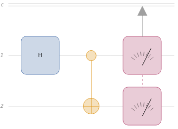
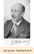
Let’s examine these operations in more detail. The gate labeled “H” is called a Hadamard gate, named after Jacques Hadamard.
What is the effect of this gate on a qubit in the register state?
Out[]=
⇒

A Quick Note on Measurement
A Quick Note on Measurement
You might wonder at what point probabilities enter the picture. Does the Hadamard gate introduce the need for probability or does the measurement? Before answering this question, what happens if the measurement is not done in the computational basis? What happens if a different measurement is performed with a special relationship to the Hadamard gate as shown below?
Performing this new measurement (not the usual computational basis) gives the same result with 100% probability after applying the Hadamard gate. Thus, there are cases where measurement also does not lead to probabilistic results.
As shown in the Bloch plot, the qubit is in a definite quantum state after the Hadamard gate is applied:
Probability is only necessary when the quantum state before measurement is not in the same basis as the measurement being performed. If you want to know precise details about this feature of quantum mechanics, it is typically expressed in terms of eigenvalues and eigenvectors of matrices. You can learn about this mathematical formalism in a course on linear algebra.
More Operations on Qubits
More Operations on Qubits
You have seen the effects of the Hadamard gate. What about the “NOT” operation?
Unsurprisingly, applying the “NOT” operation to the register state changes 0 to 1 with 100% probability.
Many important operations involve more than one qubit. One of the simplest is the “SWAP” operation. This just re-labels the qubits by swapping two of them:
Notice how the results of this circuit are always the bit sequence “10”, even though the “NOT” operation was applied to the 2nd qubit. That’s because a “SWAP” is performed just after the “NOT” operation. Contrast this with the unswapped case:
Controlled operations are another important category. One of the most common examples is the controlled not gate or “CNOT”:
On this particular input, “CNOT” does not appear to do anything. That’s because a controlled gate can be thought of like an “if” statement. If the control qubit is a “1”, perform an operation on the target qubit. If the control qubit is a “0”, do nothing.
As you can see, changing the control qubit to a “1” now results in the NOT operation being applied to the target qubit.
In the context of qubits, the CNOT gate can be used to generate quantum states with very unique properties if the control qubit is in neither the “0” nor “1” state.
The circuit above no longer results in the same measurement outcome every time. Instead, it uses a Hadamard and CNOT gate to create a state which gives “00” 50% of the time and “11” 50% of the time. This is the famous Bell state named after physicist John Bell.
Bra-Ket Notation
Bra-Ket Notation
In the formalism of quantum mechanics, how to represent and write down the various concepts is an important question. For some common quantum operations, bra-ket notation is particularly useful. This is also sometimes called Dirac notation after P.A.M. Dirac.
Below is the bra-ket notation for the NOT operation:
Example
Example
Solution
Apply the operator to the specified state:
Since the first qubit is initially in the “1” state, the target qubit (third qubit in this case) will be flipped by the controlled operation.
You can get the same result using shorthand circuit notation: