Working with Quantum Circuits
Working with Quantum Circuits
In[]:=
<<Wolfram`QuantumFramework`
Key Concepts
Key Concepts
◼
Circuit Depth
◼
Pauli Matrices
Specifying Circuits
Specifying Circuits
You have already seen many examples using the Wolfram Quantum Framework. Let’s take a moment to explicitly learn more about the framework.
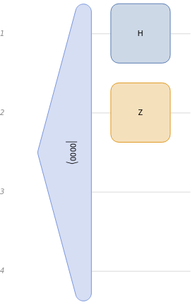
The framework supports a convenient shorthand notation for creating circuits. For example, consider the following circuit:
In[]:=
circuit1=QuantumCircuitOperator[{"0000","H"->1,"Z"->2}]
Out[]=
QuantumCircuitOperator

This is shorthand for a 4-qubit input state, a Hadamard gate on the first qubit, and a Z gate on the second qubit. You can see the diagram using the property:
"Diagram"
In[]:=
circuit1["Diagram"]
Out[]=
This circuit has no measurement operators. Thus, evaluating the circuit leads to a quantum state:
In[]:=
qs1=circuit1[]
Out[]=
QuantumState
Every quantum state has a property which shows the bra-ket (Dirac) notation:
"Formula"
In[]:=
qs1["Formula"]
Out[]=
1
2
1
2
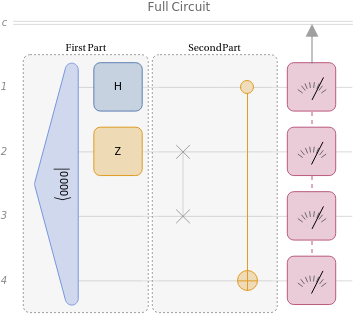
You can build up larger quantum circuits by nesting objects. The second argument can be used to label sub-circuits:
In[]:=
circuit2=QuantumCircuitOperator[{QuantumCircuitOperator[circuit1,"First Part"],QuantumCircuitOperator[{"SWAP"->{2,3},"CNOT"->{1,4}},"Second Part"],"M"->Range[4]}]
Out[]=
QuantumCircuitOperator
This can be helpful if you want to label various parts of an algorithm’s diagram:
In[]:=
circuit2["Diagram",PlotLabel->"Full Circuit"]
Out[]=
This circuit now has measurements. Thus, evaluating it leads to a measurement object:
In[]:=
mea1=circuit2[]
Out[]=
QuantumMeasurement

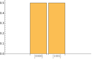
The measurement object can help you visualize the probability distribution or simply list the results:
In[]:=
mea1["Distribution"]
Out[]=
CategoricalDistribution
In[]:=
mea1["Probability"]
Out[]=
0000,1001
1
2
1
2
In[]:=
mea1["ProbabilityPlot"]
Out[]=
You can use this probability distribution to simulate measurement results if desired:
In[]:=
mea1["SimulatedMeasurement",1000]//Counts
Out[]=
|0000〉466,|1001〉534
Equivalent Operators and Circuits
Equivalent Operators and Circuits
Given the measurement distribution in the last example, you might suspect that a simpler circuit could give equivalent results. This is usually the case when designing quantum algorithms. One of the key engineering challenges for practical quantum computing is creating circuits with few enough numbers of gates to run effectively.
Let’s look at another example.
In[]:=
longops={"X"1,"X"4,"H"1,"CNOT"{2,4},"SWAP"{1,3},"Z"1};longcircuit=QuantumCircuitOperator[{QuantumCircuitOperator[longops,"Operations"],"M"->Range[4]}];longcircuit["Diagram"]
Out[]=
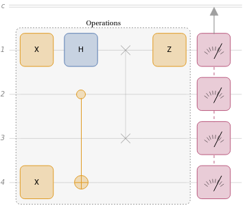
The circuit depth is the maximum number of operations performed on any qubit.
In this circuit, is it possible to come up with a different set of operations that lead to the same measurement results?
The simplicity of the measurement distribution certainly suggests this is the case. Consider the following circuit:
The circuit depth is shorter and the measurement distribution is identical:
You can even verify that the quantum state after the long sequence of operations is the same as the quantum state after the short sequence of operations:
Note that the states being equivalent before measurement is an even stronger requirement than just having identical measurement distributions.
Pauli Operators
Pauli Operators
You might have noticed that an X gate seems to act a lot like a NOT gate. That’s because they have identical effects on qubits. An X gate is a NOT gate.
Recall the Bloch sphere representation of a qubit:
Each of the six states shown above lie along the Cartesian axes of the sphere. For various historical reasons, these states have alternate names in the context of quantum computing. However, they have another interpretation in the context of linear algebra. They simply correspond to eigenvectors of the Pauli matrices:
A future lesson will discuss the matrix representation of quantum states in more detail.