Reviewing Probability
Reviewing Probability
In[]:=
<<Wolfram`QuantumFramework`
Key Concepts
Key Concepts
◼
Random outcome
◼
Probability distribution
Experiments and Randomness
Experiments and Randomness
You will no doubt be familiar with coin flips or dice as ways of generating random outcomes. For purposes of this course, you can think of a random outcome as a well defined result of some experiment. The randomness of the outcome generally means that several different outcomes were possible and there is no way to tell exactly which outcome will happen without running the experiment.
You can find much more information on probability and statistics in any of the following Wolfram U courses:
As you saw in previous lessons, the measurement outcomes of qubit states after running a quantum circuit do not always give the same results. Instead, quantum theory gives a way of computing the probability distribution for possible measurement outcomes. You can think of a probability distribution as a rule that assigns probabilities for each possible outcome of an experiment.
Let’s look at a couple examples of generating random outcomes to build intuition.
Random Numbers
Random Numbers
Suppose you want to choose a random whole number between 1 and 10. As with many concepts related to probability and statistics, there is a built-in Wolfram Language function to accomplish this:
In[]:=
RandomInteger[{1,10}]
Out[]=
8
Each time you make the random choice, the outcome will be different. You can also simulate a sequence of random choices:
In[]:=
RandomInteger[{1,10},20]
Out[]=
{9,9,9,1,4,6,5,6,1,9,3,7,10,2,1,5,9,7,6,10}
The experiment to “choose a random whole number between 1 and 10” generally assumes that random means each number has an equal probability to be chosen. Let’s look at some specific data to see that your intuitions about equal probability for outcomes must be considered carefully. You can use to give simulated random results reproducibility:
In[]:=
SeedRandom[2134];numberdata=RandomInteger[{1,10},20]
Out[]=
{5,5,7,6,5,2,6,2,9,9,5,2,10,7,10,8,9,3,2,5}
The following histogram shows some features of this outcome that may surprise you:
In[]:=
Histogram[numberdata,{.5,10.5,1},Ticks->{Range[10],Automatic}]
Out[]=
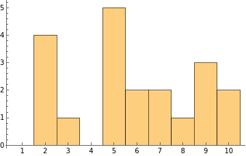
Notice that in this particular experimental outcome, the numbers 1 and 4 were not chosen at all. Also, the number five was chosen more than twice as often as you would have expected. These (perhaps) unexpected features of this particular outcome are perfectly consistent with a statistical experiment.
There is always a difference between the probability distribution of outcomes and the observed frequency of outcomes. If you repeat an experiment infinitely many times, the observed frequencies will converge to the expected distribution. However, any finite number of outcomes may display quirky features. Repeating an experiment many times is the best way to verify the expected probability distribution really does describe the experiment.
While the specifics are beyond the scope of this course, you can use functions like to see if observed outcomes match an expected distribution:
In[]:=
DistributionFitTest[numberdata,DiscreteUniformDistribution[{1,10}],"TestDataTable"]
Out[]=
Statistic | P-Value | |
Pearson 2 χ | 12. | 0.151204 |
These results can be automatically interpreted for you by the same function:
In[]:=
DistributionFitTest[numberdata,DiscreteUniformDistribution[{1,10}],"TestConclusion",SignificanceLevel->15/100]
Out[]=
The null hypothesis that the data is distributed according to the DiscreteUniformDistribution[{1,10}] is not rejected at the 15 percent level based on the Pearson test.
2
χ
See the Introduction to Statistics course for more details, but from this statistical test you can roughly conclude that 15% of all experiments following the uniform distribution of whole numbers between 1 and 10 will give outcomes this far from an observed uniform distribution. In other words, the results are really not so unusual if 15% of all experiments like this are expected to show similar patterns.
Roulette
Roulette
For many experiments, including many quantum circuits, the probabilities of various outcomes are not evenly distributed. In the game of chance called roulette, a wheel is spun, and the result will be either green, red, or black. An example roulette wheel is shown below:
Out[]=
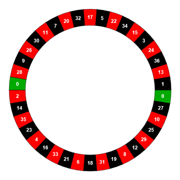
This roulette wheel has 18 red outcomes, 18 black outcomes, and 2 green outcomes. You can use the function to simulate outcomes using given weights:
In[]:=
RandomChoice[{18,18,2}->{Red,Black,Green},20]
Out[]=
,,,,,,,,,,,,,,,,,,,
With the given weights, you would expect to get roughly one green outcome out of twenty trials:
In[]:=
SeedRandom[2134];colordata=RandomChoice[{18,18,2}->{Red,Black,Green},20]
Out[]=
,,,,,,,,,,,,,,,,,,,
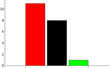
As with the random number example, notice that the observed frequency in these particular trials is not equal for red and black, even though they have the same probability according to the distribution:
In[]:=
colorcounts=Counts[colordata];BarChart[Values@colorcounts,ChartStyle->Keys@colorcounts]
Out[]=
In fact, the P-value closer to 1 indicates that this sample variation away from the overall distribution is quite typical:
In[]:=
DistributionFitTest,"TestDataTable"
Out[]=
Statistic | P-Value | |
Pearson 2 χ | 0.477778 | 0.787502 |
Thus, this statistical test indicates you should not reject the hypothesis that the simulated roulette results came from the theoretical roulette distribution:
In[]:=
DistributionFitTest,"ShortTestConclusion"
Out[]=
Do not reject
Roulette Extension
Roulette Extension
As a further exploration of the roulette example, what is the probability for getting green results on 20 spins of the roulette wheel? You can use the Wolfram Language’s support for probability and statistics to compute the answer without resorting to formulas. However, the Wolfram U courses linked at the beginning of the lesson are excellent resources for getting a complete introduction to probability.
k
Compute the probability of getting a green result on a single spin of the wheel:
In[]:=
Probability[x==Green,xEmpiricalDistribution[{18,18,2}->{Red,Black,Green}]]
Out[]=
1
19
A binomial distribution can be used to model repeated trials where there are successes and failures with given probability (in this case, green and not-green):
In[]:=
NProbability[k==1,kBinomialDistribution[20,1/19]]
Out[]=
0.376821
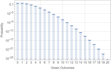
The computation above shows that approximately 37.7% of all samples with 20 spins of the wheel should get exactly one green result. You can plot the probabilities for other numbers of green outcomes in 20 trials as well:
In[]:=
DiscretePlotPDF[BinomialDistribution[20,1/19],k],{k,0,20},//Rasterize
Out[]=
Alternatively you could use a multinomial distribution to reach the same conclusion by considering all three categories:
Testing Coins
Testing Coins
Suppose that you want to determine whether or not a coin is fair. One way to do this is simply record the results of many outcomes. Record 1 if the outcome is heads and 0 if the outcome is tails. The following code simulates twenty trials:
In this case, the observed frequencies did match the probabilities from the distribution of a fair coin:
Given the observed data, you can compute the likelihood of those observations, as a function of the coin’s probability to give heads. Since this sample had the same observed frequencies as the fair coin distribution, the maximum-likelihood estimate for the chance to give heads is 50%:
The following animation shows how the maximum-likelihood estimate for the probabiity to obtain heads changes as you accumulate more trials in this simulation. In practice, you should always fix the number of trials before conducting such a statistical test:
Notice how the curve representing likelihood gets more “narrow” in the previous animation. That’s because the standard error for estimating the coin’s true probability distribution decreases with the number of trials:
As the number of trials increases, the standard error in estimating the coin’s true distribution will tend to zero:
While you may be interested in estimating the maximum-likelihood fit for measurement distribution parameters, the relevant question for this example is whether the sample data is consistent with a fair coin or whether the sample data is highly unlikely to be produced by a fair coin.
As before, you can test whether or not you should reject the hypothesis that the coin is fair:
The plot below shows that the probability of observing this particular sample data never falls below the given significance threshold as more trials accumulate:
You can simulate a biased coin with 60% probability to give heads as follows:
This time, sufficiently many trials will allow you to differentiate between the biased coin and a fair coin. It is good practice to fix the number of trials before proceeding to collect data for a statistical test of this variety.
In summary, experiments with quantum systems will generally give results which follow a measurement distribution that can be theoretically computed. To see if the results are really consistent with the theoretical prediction, the experiment must be carried out for many trials to build statistical confidence in the answer.
In future lessons, you will see some quantum algorithms which are not guaranteed to give a correct solution, but will give a correct the solution with high probability. In such cases, you must then consider not only the quantum algorithm, but also the practical considerations of repeating the algorithm multiple times to verify the solution.