Superposition and Entanglement
Superposition and Entanglement
In[]:=
<<Wolfram`QuantumFramework`
Key Concepts
Key Concepts
◼
Superposition
◼
Entanglement
◼
GHZ state
◼
Partial Trace
◼
Mixed State
◼
Pure State
Superposition and Entanglement
Superposition and Entanglement
Quantum superposition and quantum entanglement are terms you may have heard often in popular culture.
A superposition is simply a quantum state which is not in any state in the measurement basis. Instead, it is in a linear combination of more than one basis state. You have seen many such states represented as vectors.
A uniform superposition has equal chance to give each basis state when measured:
In[]:=
QuantumState["UniformSuperposition"]["Formula"]
Out[]=
1
2
1
2
Consider the 2-qubit uniform superposition state:
In[]:=
QuantumState["UniformSuperposition"[2]]["Formula"]
Out[]=
1
2
1
2
1
2
1
2
This state is equivalent to each of the single qubits being in a uniform superposition as well:
In[]:=
nonentangled=QuantumTensorProduct[QuantumState["UniformSuperposition"],QuantumState["UniformSuperposition"]]
Out[]=
QuantumState
In[]:=
nonentangled==QuantumState["UniformSuperposition"[2]]
Out[]=
True
In[]:=
nonentangled["Formula"]
Out[]=
1
2
1
2
1
2
1
2
Since each qubit in this state can be represented as its own independent state (by the tensor product construction), there is no entanglement present in this state.
In[]:=
QuantumEntangledQ[nonentangled]
Out[]=
False
Entanglement describes a quantum system in which parts of that system cannot be given complete, independent descriptions. In other words, the whole system has a definite state, but some individual parts may not have a definite state.
This may sound exotic, however it is relatively straightforward to create entangled quantum states. Consider the following circuit:
In[]:=
sameEntangler=QuantumCircuitOperator[{"H"->1,"CNOT"->{1,2}}]
Out[]=
QuantumCircuitOperator
When applied to the register state, this circuit will create the famous Bell state:
In[]:=
entangled=sameEntangler[]
Out[]=
QuantumState
In[]:=
entangled==QuantumState["Bell"]
Out[]=
True
In[]:=
entangled["Formula"]
Out[]=
1
2
1
2
Unlike the tensor product state leading to a uniform superposition, the only possible measurement outcomes for this state are “00” or “11”.
In[]:=
entangled["ProbabilitiesPlot"]
Out[]=
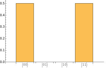
Before measuring the Bell state, what can you say about the individual qubit states? In some sense, you might be able to say that each qubit is in “the same” state. But what is that state? Until it is measured, you don’t know if they are both “0” or both “1”. But you do know the results will be identical when measuring each qubit in this state.
This certainty about measurement correlations that still leave the individual states in question is the hallmark of entanglement.
In[]:=
QuantumEntangledQ[entangled]
Out[]=
True
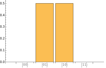
The following circuit also creates entanglement, but this time the results of each qubit are opposites:
In[]:=
oppositeEntangler=QuantumCircuitOperator[{"H"->1,"C0NOT"->{1,2}}]
Out[]=
QuantumCircuitOperator
Apply the circuit:
In[]:=
entangled2=oppositeEntangler[]
Out[]=
QuantumState
Check for entanglement:
In[]:=
QuantumEntangledQ[entangled2]
Out[]=
True
Visualize the results:
In[]:=
entangled2["Formula"]
Out[]=
1
2
1
2
In[]:=
entangled2["ProbabilitiesPlot"]
Out[]=
GHZ States
GHZ States
Entanglement can extend beyond only two qubits. The GHZ circuit is shown below:
In[]:=
QuantumCircuitOperator["GHZ"]["Diagram"]
Out[]=
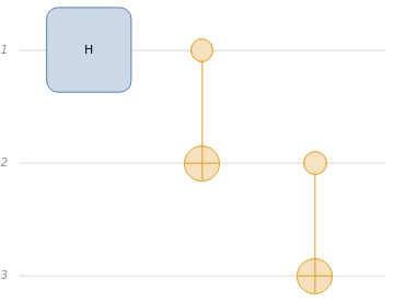
This circuit creates a state in which the measurement of all qubits will be perfectly correlated, but you can’t tell the result before measuring:
In this case, all three qubits share in the entanglement:
Such a state is called a GHZ state. The GHZ type states can be extended to any number of qubits:
Partial Traces
Partial Traces
Earlier in the lesson, you may have wondered what can be said about a qubit which is entangled with other qubits. Surely it must be possible to assign some kind of state to that qubit. Subsystems of a larger quantum system can be assigned states through the mathematical operation known as a partial trace.
The result is a quantum state. This state is the same as the uniform superposition:
That result should be expected since the non-entangled state was a tensor product state by construction.
But what happens if we try the same procedure with the entangled state?
The result is no longer simply the uniform superposition state:
In fact, it is a type of state which has not appeared in this course previously.
This formula appears strange, because a single qubit from a bell pair must be described by what is known as a mixed state.
This is in contrast with states known as pure states:
The difference is subtle. A pure state can be represented by a state vector, which means a pure state is a definite linear combination of basis vectors. Depending on your measurement basis, you may not get the same result every time; however, linear algebra results guarantee there will be some measurement basis in which you can get the same result every time.
In contrast, a subsystem in a mixed state has inherent uncertainty built into the subsystem. You cannot find a measurement basis for the subsystem alone which will guarantee the same result every time. That’s because entanglement implies that the subsystem shares information with some larger system.
For example, the Bell pair of qubits share the information that they will either both give “0” or both give “1”. However, there is an equal chance of either result, giving some inherent uncertainty about the single qubit states.
The mixed single-qubit has 1 bit of entropy:
The pure single-qubit has 0 bits of entropy:
The mixed-state single qubit can be “purified” by considering it as part of a larger system:
It should not surprise you that the larger, purified state is none other than the Bell state you started with:
Even though the mixed and pure single-qubit states differ in this very important property, the probability distributions for the single qubit are identical:
It is only by measuring the full system (the first and second qubits in this case) that entanglement can be seen in the correlations:
You can also see the difference between mixed and pure single-qubit states from their Bloch plots:
In contrast, this mixed state is precisely in the middle of the Bloch sphere:
No matter which basis you choose to measure this qubit, you are guaranteed uncertainty. Such a state is known as a uniform mixture: