Wolfram Cloud Document

Bernstein-Vazirani Algorithm

In[]:=

<<Wolfram`QuantumFramework`

Key Concepts

◼

Oracle function

◼

Bernstein-Vazirani problem

Statement of the Bernstein-Vazirani Problem

In many computer science problems, it is common to assume there is some kind of oracle function that is used in order to compute partial results for use in the rest of an algorithm. In practice, the oracle could be a database query or some similar operation.

The Bernstein-Vazirani problem involves using an oracle to discover a secret code sequence. The problem can be stated as follows:

◼

There is a secret sequence,

, of length

, consisting of ones and zeros. Formally,

s∈

{0,1}

◼

There is an oracle,

, which accepts a sequence,

, of length

and returns the dot product of

and

modulo 2. Formally,

{0,1}

↦{0,1}

such that

f(x)=x·smod2

◼

The goal is to find the secret sequence,

, with as few uses of the oracle function as possible.

The classical oracle function can be implemented in a straightforward way:

In[]:=

bvClassicalF[x_List,s_List]:=Mod[x.s,2]

See if you can use this oracle function and a classical algorithm to discover the following secret code:

In[]:=

secret=

;

In[]:=

Length[secret]

Out[]=

Classical Bernstein-Vazirani Solution

You may have tried several different methods, but discovering the secret sequence of length

will require at minimum

queries to the classical oracle. The solution can be obtained by querying the oracle with each possible sequence that has exactly one 1 and the rest 0:

In[]:=

Module{queries,res,counter},queries={{1,0,0},{0,1,0},{0,0,1}};counter=0;Tableres=bvClassicalF[q,secret];

Echo[

]

;res,{q,queries}

first query: {1, 0, 0} ⇒ result: 1

second query: {0, 1, 0} ⇒ result: 0

third query: {0, 0, 1} ⇒ result: 1

Out[]=

{1,0,1}

In[]:=

{1,0,1}==secret

Out[]=

True

If you want to try your own algorithms, you can generate a new secret sequence as follows:

In[]:=

newsecret=RandomChoice[Tuples[{0,1},3]]//Iconize

Out[]=

In[]:=

Length[newsecret]

Out[]=

Quantum Bernstein-Vazirani Algorithm

In the quantum version of the algorithm, the oracle will also depend on the secret sequence. This is no different from the classical oracle.

In order to create the quantum BV oracle for secret sequence of length

, you will need

n+1

qubits. For each 1 in the secret sequence, the oracle applies a CNOT gate with control qubit corresponding to that one’s place in the secret sequence and target qubit corresponding to the

n+1

qubit.

Recall the secret sequence from before:

In[]:=

secret

Out[]=

{1,0,1}

The quantum BV oracle for this sequence is given by:

In[]:=

QuantumCircuitOperator["BernsteinVaziraniOracle"[secret]]["Diagram",ImageSize->Small]

Out[]=

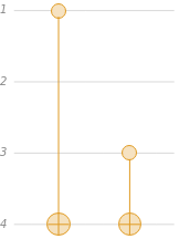
In the context of the problem, you might imagine that this oracle is a quantum device which is networked to the rest of your circuit but which you cannot directly “see” (otherwise the gate structure of the oracle immediately gives away the answer).

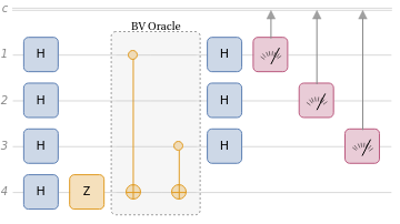
In order to use this oracle to discover the secret code, only one query is necessary. Using the phenomenon of phase kickback, it is possible to send a uniform superposition of all possible sequences (as measured in the computational basis) and encode the solution in the three control qubits.

The full circuit would look like this:

In[]:=

QuantumCircuitOperator["BernsteinVazirani"[secret]]["Diagram"]

Out[]=

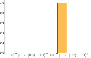
The algorithm gives the secret code in only a single query:

In[]:=

QuantumCircuitOperator["BernsteinVazirani"[secret]][]["ProbabilitiesPlot"]

Out[]=

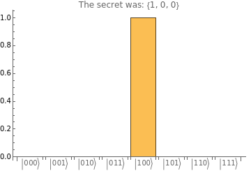
Try again with some randomized secret codes:

In[]:=

newsecret=RandomChoice[Tuples[{0,1},3]];QuantumCircuitOperator["BernsteinVazirani"[newsecret]][]["ProbabilitiesPlot",PlotLabel->StringJoin["The secret was: ",ToString@newsecret]]

Out[]=

Effects of Noise

While solving the problem in only a single query to the quantum oracle is possible theoretically, real quantum circuits involve some errors caused by various effects. All of the previous circuits you have considered did not take this phenomena into account.

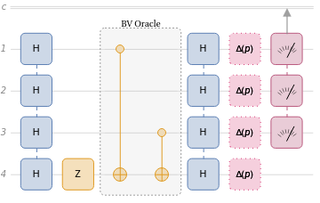
The following circuit defines the BV algorithm but introduces a noise channel just before the measurements can be performed. You might imagine this noise is from imperfect measurement or from the cumulative effect of previous errors in the circuit.

In[]:=

noisyBV[s_List]:=With[{n=Length[s]},QuantumCircuitOperator[{"H"->Range[n+1],"Z"->n+1,QuantumCircuitOperator["BernsteinVaziraniOracle"[s],"BV Oracle"],"H"->Range[n+1],Splice@Table[QuantumChannel["Depolarizing"[p],{k}],{k,n+1}],"M"->Range[n]},"Parameters"->p]]

A noisy version of the previous circuit might look like this:

In[]:=

noisyBV[secret]["Diagram"]

Out[]=

Notice that the measurement distribution now depends on the probability of the noise channels affecting each qubit:

If the so-called depolarizing noise channels affect the qubits with probability under 5%, the chance of returning the secret code is still quite high:

The following animation shows the effect of increasing the depolarizing probability:

You can also plot all measurement outcome probabilities as a function of the depolarizing probability:

However, you should note that the probabilities of outcomes with identical Hamming distance away from the secret code are the same:

This plot shows the probabilities of outcomes that are a given Hamming distance from the secret code:

Compensating for Errors

In practical quantum algorithms, an important consideration is the resilience of that algorithm to errors. Let’s use the noisy circuit in the last section for an example of a very simple error mitigating scheme.

First, compute the distribution of measurement outcomes for this circuit:

The probability of success on each run of the circuit can be obtained:

Using a little probability theory, the chance of half or more of the runs failing can be computed as:

That mathematical function might look a little scary, but you can easily work with it using the Wolfram Language. It can be used like any other symbol. The plot below shows contours which relate the probability this simple error mitigation scheme failing to the probability of depolarization:

Notice that increasing the number of trials in this error mitigation scheme generally reduces the probability for the scheme to fail, even if the probability of depolarization is quite high.

The number of trials in which you run a quantum circuit is often called the number of “shots” by hardware providers. Keep in mind that any circuit which can give different results on different trials must be run more than once in order that you get a good estimate of the true measurement distribution.