MAM2046W - Second year nonlinear dynamics

Section 2.3: The Poincaré-Bendixson theorem

We actually already touched on this in section 1.2 but we are going to look at it in much more detail now. This will allow us to show that there exist closed orbits, as opposed to the previous section where we were finding methods to show that there were no closed orbits.

The Poincaré-Bendixson theorem says that when certain criteria are fulfilled, we are guaranteed a closed orbit. These criteria are (don’t worry too much about the terms in bold):

1) We have some closed, bounded subset of



, call it

2) We have some vector field which is continuously differentiable on an open subset of

3) There are no fixed points of the vector field within

4) There is some trajectory,

, which is completely confined within

Then

could

either itself be a closed orbit, or it must approach some closed orbit in

t->∞

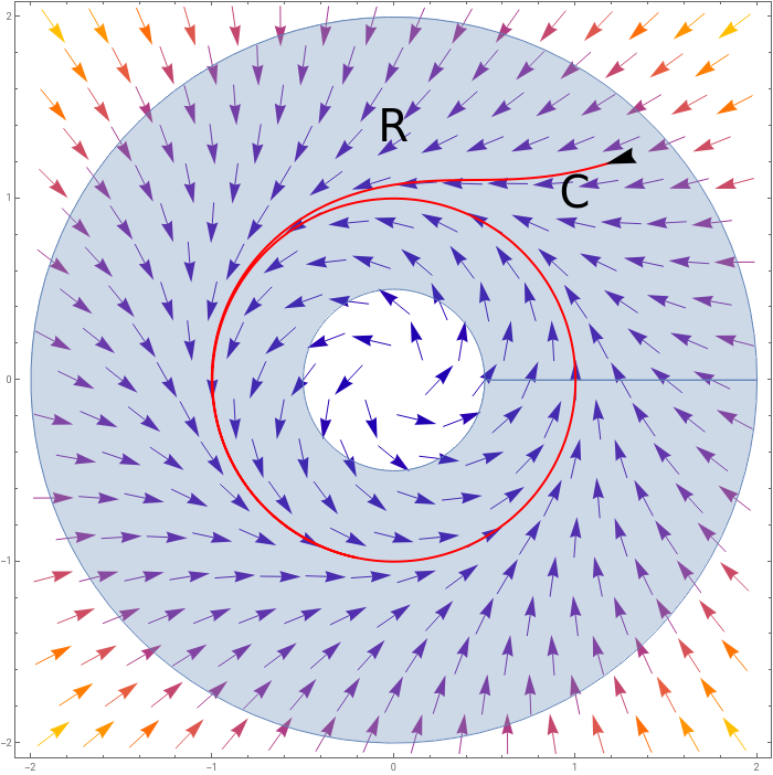
Note very importantly that when we say that there are no fixed points in

this doesn’t mean that there can be no fixed points inside the closed orbit. This sounds very strange at first, but

could, for instance have a piece taken out of the middle of it, where the fixed point exists. For example:

In[]:=

eqns=SimplifySolveD

x[t]

y[t]

,t==

(

x[t]

y[t]

)

(1-(

x[t]

y[t]

)),DArcTan

y[t]

x[t]

,t==1,{x'[t],y'[t]}[[1]];startpoints={{1.2,1.2}};({x[t],y[t]}/.NDSolve[{x'[t]==(x'[t]/.eqns),y'[t]==(y'[t]/.eqns),x[0]==#[[1]],y[0]==#[[2]]},{x,y},{t,0,10}][[1]])&/@startpoints;Show[VectorPlot[Evaluate[{x'[t],y'[t]}/.eqns/.{x[t]->x,y[t]->y}],{x,-2,2},{y,-2,2}],ParametricPlot[r{Cos[θ],Sin[θ]},{θ,0,2π},{r,0.5,2},PlotPoints->100],ParametricPlot[%,{t,0,10},PlotStyle->{{Red,Thick},{Red,Thick},{Red,Thick},{Red,Thick},{Blue,Thick},{Blue,Thick},{Blue,Thick},{Blue,Thick}}],Graphics[Arrow[{#/.t->0,#/.t->0.01}]]&/@%,Graphics[Text[Style["R",40],{0,1.4}]],Graphics[Text[Style["C",40],{1,1.03}]],ImageSize->700]

Out[]=

Here we have a region

(the blue shaded region) which is closed and bounded (think of it as being a finite region which has a border), where the vector field is continuously differentiable on an open subset of

(ie. it doesn’t have to be differentiable on the boundary itself). We have a curve

which is always within

. There are no fixed points in

. This means that we are guaranteed that there will be a closed orbit, and indeed the closed orbit is the one which

tends to as

t->∞

In fact we will always have a hole in the middle, because if there is a closed orbit then there must be a fixed point within it, so we have to exclude that from

by cutting a hole out of it.

There’s something that we should note about the vector field in the above example. On the boundary of the region

the vector field is always pointing in. This means that once you are in, you’re in. You can’t escape the region, because any trajectory which left the region would have a vector pointing out of it.

This is the whole trick to finding the right region such that we have a trajectory which is always within that region. Such a region is called a trapping region.

So long as we can find a trapping region, and we can make sure that there are no fixed points within that region, then we are sorted.

Example

Here we will be able to find a trapping region by looking carefully at the vector field. The equation in question is similar to the previous one, but with an extra term, parameterised by a constant μ. Again we are looking at polar coordinates:



=r(1-

)+rμcosθ



μ here is a constant and we will look at it for positive values only (negative values are the same as letting

θ->θ+π

The question is whether we can find some region with an inner radius for which



is always positive, and an outer radius where



is always negative. Note that here we are just trying to find a perfect annulus. The bounding region doesn't have to be, but we will look for such a region here.

We want to find

min

for which:

min

(1-

min

μcosθ>0

For all values of θ. Solving for

min

gives

min

1+μcosθ

What is the lowest value that the right hand side can take? Well, the minimum value of cos θ is -1, so we can be sure that

min

1-μ

So we can always be sure that on a circle of

min



will be positive. To play it safe, let’s set

min

=0.9

1-μ

We see here that with our stricter bound, we are constrained to

μ<=1

, and in fact we have to exclude μ=1 as well because with μ=1,

min

and there is a fixed point there, so we can’t include it. So we are only looking at cases for which

μ<1

Now running through the same argument for

max

for which we have to have



negative you should find

max

1+μ

and again we can set

max

=1.1

1+μ

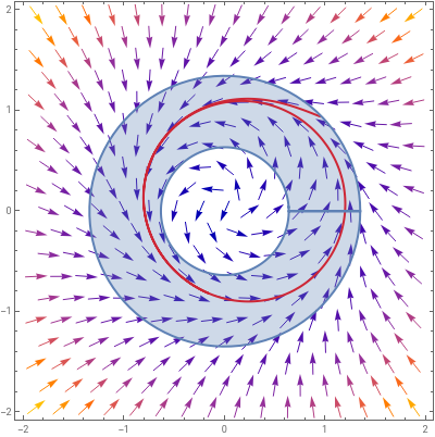
In the following we animate over different values of μ from 0 to 1. You can see that the arrows don’t shift so much other than in the top right corner as μ changes. We look at a trajectory that starts just inside the region and note that it is always contained within our annulus of radius

0.9

1-μ

<r<1.1

1+μ

In[]:=

pl[μ_]:=Module{eqns,startpoints},eqns=SimplifySolveD

x[t]

y[t]

,t==

(

x[t]

y[t]

)

(1-(

x[t]

y[t]

))+μ

(

x[t]

y[t]

)

x[t]

(

x[t]

y[t]

)

,DArcTan

y[t]

x[t]

,t==1,{x'[t],y'[t]}[[1]];startpoints=1.09

(1+μ)



;sol=({x[t],y[t]}/.NDSolve[{x'[t]==(x'[t]/.eqns),y'[t]==(y'[t]/.eqns),x[0]==#[[1]],y[0]==#[[2]]},{x,y},{t,0,20}][[1]])&/@startpoints;Show[VectorPlot[Evaluate[{x'[t],y'[t]}/.eqns/.{x[t]->x,y[t]->y}],{x,-2,2},{y,-2,2}],ParametricPlot[sol,{t,0,10},PlotStyle->{Red,Thick}],ParametricPlot[r{Cos[θ],Sin[θ]},{θ,0,2π},r,0.9

1-μ

,1.1

1+μ

,PlotPoints->100,BoundaryStyle->Thick],ImageSize->400]Table[pl[μ],{μ,0,0.95,0.05}];ListAnimate[%,SaveDefinitions->True]

Out[]=

Indeed we can see that the trajectory is always within the annulus that we have created, and that there does appear to be a limit cycle.

Example

Let’s look at another example, this time a bit more real-world inspired, and a little more complex.

The equations modelling this system are:

So, the question is whether we can find a trapping region in the phase space which does not contain any fixed point.

I’m actually just going to give you the outer trapping region, as the argument for why it is a reasonable trapping reason is a little naunced, and not very enlightening.

It turns out that the following region is a reasonable trapping region:

It might not look like the arrows along the bottom are all pointing into the region, but this is an artifact of where the vectors are sampled. If you look along the x-axis you see that

So is that enough to prove that we have a closed orbit? Not yet, we have to have a trapping region with no fixed points, but there is a fixed point in this system at:

We first have to find the Jacobian of our system:

The fixed point is at

So the Jacobian at this point is:

The determinant and trace of this are:

Let’s remind ourselves once more of the possible behaviours in 2d linear systems:

It actually doesn’t matter whether the fixed point is a node or a spiral, just whether or not it’s stable or unstable, so we only need to know whether τ is greater than or less than 0. The dividing line between the two is going to be when

Which is given by

To see which is which, we let a=0, b=0.5 and see that τ=0.75, which implies that the region shaded in blue corresponds to unstable spirals/nodes. If we have an unstable node/spiral, we can excise this region from the trapping region, and will end up with arrows pointing into the trapping region, therefore the shaded region is the region of closed orbits:

We should have convinced ourselves earlier that all vectors are necessarily pointing vertically along the x-axis, but it doesn’t look like it in this plot. This again is an artifact of where the vectors are sitting. Zooming in on the x-axis we see:

which should convince ourselves that all is well.

However, excising a small disk around the fixed point, all is not well:

Not all vectors are pointing out. This is because this is an unstable spiral, so we would actually have to choose a differently shaped excising region in order to have all vectors pointing out of it. We will simply have to convince ourselves for now that because this is an unstable spiral, we could in theory find an appropriate region. It will be some sort of ellipse-like shape at a slight angle.

Now let’s look at two trajectories for this system, starting inside the trapping region:

and finally, numerically, I hope that we can believe that we do indeed have a closed orbit!

Lack of chaos in 2d

So, what we have found is that given a relatively simple constraint: trajectories bounded in some region, where there are no fixed points in the region, there is only one thing that can happen: all trajectories end up being attracted to a closed orbit. There’s no sensitivity to initial conditions, that if you change the initial conditions a little, you will end up somewhere completely differently.

And if it’s not confined to a closed bounded region? Well then it will go off to infinity - also not so interesting.

And if there is a fixed point that can’t be excised? Well then trajectories will all end up there.

In fact this statement shows that there can be no chaos in 2d. Given some dynamical system in some bounded region, there’s only a very limited number of things that can happen. This can be seen rather intuitively by the fact that trajectories can’t cross each other, so in 2d, everything is pretty constrained. In 3d however there is suddenly so much more space for the trajectories to move, and indeed in 3d (and above) you can have chaos. In 3d the Poincaré-Bendixson theory does not hold, and so you have behaviours which are much more complex than closed orbits there.

As a caveat, we have to be a little careful with the above statement, as it necessitates a smooth, continuous vector field. Throw singularities into the problem and all sorts of crazy stuff can happen. Similarly, if you are talking about difference equations, and not differential equations, you can have chaos even in 1D.

Other ways of finding limit cycles

This is an example taken from the exercises of section 7.3 of Strogatz, and it gives a nice alternative way of showing that there is a limit cycle.

Given the vector field given by

How can we show that there is a limit cycle here? Well, we can do this by constructing a function given by:

whose time derivative is:

We can easily linearise our system at the origin and it gives us:

Which you can show easily gives you an unstable spiral. So if we start anywhere, then we are going to move towards the ellipse given by

Homepage