In today' s episode of perovskite mythbusters ... we investigate the possibility of non - ideality of mixing of GBL and FAH. If one mixes unit volumes of the two species, is the resulting volume different than two units of volume? Using a series of liquid handler experiments performed at ECL, and volume determination by ultrasonic height measurement and image analysis, we bound the effect to be <2% over the entire range of GBL/FAH ratios; this bound is determined by limits on our ability to dispense and measure. Therefore we conclude that the assumption of ideal mixing volume is not a significant source of error in our perovskite experiments, but this could be better studied using a proposed bench-scale experiment.
Rough Notes from gathering from ECL Experiments
Rough Notes from gathering from ECL Experiments
Rough plots examining the initial 50% v/v data (with varying volume size)
Rough plots examining the initial 50% v/v data (with varying volume size)
Analysis
Analysis
Brief description of the experiment: GBL and FAH were dispensed using a Hamilton STARLET liquid handler at ECL, using 300 uL tips and the default pipetting methods into our favorite glass vials. In addition to performing ultrasound measurements of the dispensed heights, I also used the vial images and extract the pixel positions of the top of the glass vial, the bottom of the meniscus, the bottom of the glass vial, and the left and right walls of the glass vials. Many of these experiments do not have data on the vial top, because these were cut off. Most dispenses were performed as two dispense operations (e.g., 250 uL + 250 uL), except for the cases of 25% FAH and 75% FAH which used three dispenses (250 uL + 125 uL + 125 uL). The Ultrasound volume measurements have had some problems, so in a couple of cases we only have gravimetric estimates (from vial weight) of the dispensed volumes (in principle these are more precise, but they are a different type of measurement)
Import the data
Import the data
In[]:=
SetDirectory@NotebookDirectory[];data=SemanticImport["2019.06.11_dataset.xlsx"]
Out[]=
Comment: Observed volume for Object[Sample,StockSolution, “id1ZA60vLPkj5P”] is probably erroneous (I suspect it is using the nominal specification as the measurement failed). For some of the points I was able to perform duplicate ultrasound measurements.
How well does the observed meniscus position in images relate to nominal and ultrasound volumes?
How well does the observed meniscus position in images relate to nominal and ultrasound volumes?
Helper functions for data processing and visualization
Helper functions for data processing and visualization
Relate image observation to nominal volume specification
Relate image observation to nominal volume specification
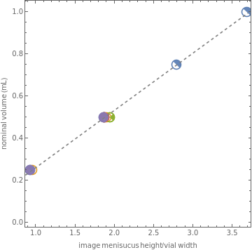
pixelToNominalVolume=LinearModelFit[QuantityMagnitude@Normal@data[All,calibrateVolume["nominal volume"]],{p},p]visualizeFit[data,pixelToNominalVolume,"nominal volume"]%%["SinglePredictionConfidenceIntervalTable"]
Out[]=
FittedModel
Out[]=
Out[]=
Observed | Predicted | Standard Error | Confidence Interval |
1. | 0.991046 | 0.0113464 | {0.966073,1.01602} |
0.5 | 0.498608 | 0.00942716 | {0.477859,0.519357} |
0.75 | 0.747121 | 0.0099483 | {0.725225,0.769017} |
0.5 | 0.497766 | 0.00942719 | {0.477017,0.518515} |
0.25 | 0.241362 | 0.00999658 | {0.21936,0.263365} |
0.5 | 0.505482 | 0.00942741 | {0.484733,0.526232} |
0.25 | 0.249319 | 0.00996301 | {0.22739,0.271247} |
0.5 | 0.517624 | 0.00942987 | {0.496869,0.538379} |
0.5 | 0.517624 | 0.00942987 | {0.496869,0.538379} |
0.5 | 0.497399 | 0.00942721 | {0.47665,0.518148} |
0.5 | 0.498396 | 0.00942717 | {0.477647,0.519145} |
0.25 | 0.242163 | 0.00999316 | {0.220168,0.264158} |
0.5 | 0.49609 | 0.00942728 | {0.475341,0.516839} |
Relate image observation to ultrasound volume measurements
Relate image observation to ultrasound volume measurements
Comment: We don’t have ultrasound measurements for all points, so delete missing cases.
In[]:=
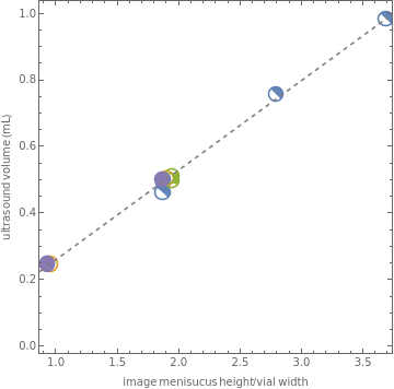
pixelToUltrasoundVolume=LinearModelFit[DeleteCases[{_,_QuantityMagnitude}]@QuantityMagnitude@Normal@data[All,calibrateVolume["ultrasound volume"]],{p},p]visualizeFit[data,pixelToUltrasoundVolume,"ultrasound volume"]%%["SinglePredictionConfidenceIntervalTable"]
Out[]=
FittedModel
Out[]=
Out[]=
Observed | Predicted | Standard Error | Confidence Interval |
0.985354 | 0.984446 | 0.0162443 | {0.948251,1.02064} |
0.50174 | 0.496149 | 0.0135101 | {0.466047,0.526251} |
0.758387 | 0.742572 | 0.0142519 | {0.710817,0.774327} |
0.494851 | 0.495313 | 0.0135101 | {0.465211,0.525416} |
0.25 | 0.241066 | 0.0143223 | {0.209154,0.272978} |
0.505538 | 0.502965 | 0.0135104 | {0.472862,0.533068} |
0.248586 | 0.248955 | 0.0142744 | {0.21715,0.280761} |
0.5122 | 0.515004 | 0.0135139 | {0.484893,0.545115} |
0.499498 | 0.515004 | 0.0135139 | {0.484893,0.545115} |
0.464307 | 0.49495 | 0.0135102 | {0.464847,0.525052} |
0.249098 | 0.24186 | 0.0143174 | {0.209959,0.273761} |
0.502377 | 0.493652 | 0.0135103 | {0.463549,0.523755} |
Conclusion: The image based determinations of volume are well correlated to the nominal and ultrasound volumes over this range. They reproduce these with standard error of 0.009 and 0.015 mL, respectively. The error of the former is in line with our expectations about the error in our liquid handler dispense volumes (note that each of these used two dispenses, except for the volume fraction 0.25 and 0.75 which use 3 dispenses)
Random out-takes
Random out-takes
Look for evidence of deviations from ideal mixing volumes
Look for evidence of deviations from ideal mixing volumes
Define helper functions and look at data
Define helper functions and look at data
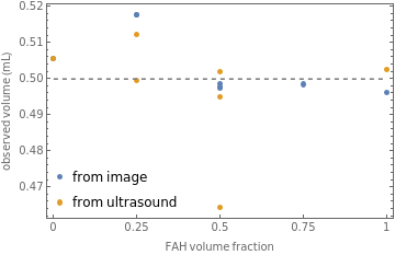
How do observed volumes vary as a function of FAH volume fraction, for a fixed nominal volume of 0.5 mL?
How do observed volumes vary as a function of FAH volume fraction, for a fixed nominal volume of 0.5 mL?
In[]:=
With[{constantNominal=data[Select[#["nominal volume"]Quantity[0.50,"Milliliters"]&],All]},With[{imageVolume=constantNominal[All,comparePredictionWithFraction[pixelToNominalVolume[imageVolume[#]]&]]//DeleteCases[{_,_Missing}],ultrasoundVolume=constantNominal[All,comparePredictionWithFraction[Lookup[#,"ultrasound volume"]&]]//DeleteCases[{_,_Missing}]},Show[ListPlot[{imageVolume,ultrasoundVolume},PlotRangeAll,FrameTrue,FrameLabel{"FAH volume fraction","observed volume (mL)"},FrameTicks{Automatic,{{0,0.25`,0.50`,0.75`,1},None}},PlotLegendsPlaced[{"from image","from ultrasound"},{Left,Bottom}]],Plot[0.5,{x,0,1},PlotStyle{Gray,Dashed}]]]]
Out[]=
Comments: Dashed horizontal line indicates the target nominal total volume. The volume fraction 0, 1, and 0.5 use two dispenses. The 0.25 and 0.75 points use three dispenses. The “image” and “ultrasound” points for FAH volume fraction = 0 are on top of each other (image volume = 0.5054 mL versus ultrasound = 0.5055); also, we don’t have an ultrasound measurement for 0.75). Based on our calibration data, we should expect ~ 0.010 mL error bars on the image data. If we assume that dispense errors are normally distributed, then the fact that we are 1-2 sigma away for the 0.25 volume fraction sample (with 3 dispenses) is pretty reasonable. I have no idea what’s up with the one goofy 0.5 point, and would just attribute this to noise on the ultrasound measurement.
Conclusion: There is no compelling evidence for significant non-ideality of mixing. Any deviations from ideal mixing volume for GBL and FAH appear to be below the limits with which we can dispense and measure by this approach (0.01 mL/0.50mL = 2%). If we really want to nail this down, I suggest a laboratory experiment using a graduated cylinder and burette. Using a Class-A IN graduated cylinder and Class-A EX burette, perform one experiment dispensing GBL into FAH and one experiment vice-versa, recording the volumes in the graduated cylinder and burette at each step. (be sure to mix). Could be a fun afternoon for a careful undergraduate student.
Conclusion: There is no compelling evidence for significant non-ideality of mixing. Any deviations from ideal mixing volume for GBL and FAH appear to be below the limits with which we can dispense and measure by this approach (0.01 mL/0.50mL = 2%). If we really want to nail this down, I suggest a laboratory experiment using a graduated cylinder and burette. Using a Class-A IN graduated cylinder and Class-A EX burette, perform one experiment dispensing GBL into FAH and one experiment vice-versa, recording the volumes in the graduated cylinder and burette at each step. (be sure to mix). Could be a fun afternoon for a careful undergraduate student.
Another look...directly at the images without an intermediate function.
Another look...directly at the images without an intermediate function.
Motivation: One might argue that the fit to ultrasound height or fit to nominal volume is skewing the measurement. So here instead we look directly at the observed height of the meniscus (normalized by the constant vial width) to eliminate any possibility of artifacts. This makes the dependent axis in terms of a ratio with some unknown relationship to volume.
We can then compute the variation above the mean. It is 2-3% consistent with the estimates above.
Conclusion: This confirms the previous claims that the observed variation is small.


