1 | Points and vectors
1 | Points and vectors
This chapter of Multivariable Calculus by Dr JH Klopper is licensed under an Attribution-NonCommercial-NoDerivatives 4.0 International Licence available at THE CREATIVE COMMONS .
1.1 Introduction
1.1 Introduction
Vectors form a central part of the study of multivariable and vector calculus. Vectors, vector spaces, and matrices form a central part of the study of linear algebra and we will learn many of their properties.
We begin our study here, by looking at vectors. You might be familiar with vectors from physics, where they denote a magnitude and a direction, i.e. a force or velocity or acceleration. There are a lot more to vectors, though. Before we dive in, we will start with the very familiar concept of points in the plane.
1.2 Points
1.2 Points
Definition 1.2.1 The Euclidean plane or the Cartesian plane is the -dimensional -plane that holds rectangular coordinates as tuples of numbers, , where both . By convention, these two points indicate a and a value on the correspondingly named perpendicular axes.
2
xy
(x,y)
x,y∈
x
y
We use the term Euclidean to indicate a system in which the rules of Euclidean geometry holds.
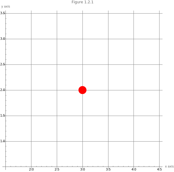
Definition 1.2.2 A point is usually written as an uppercase letter and a subscript in the range if there are subsequent points. The tuple follows directly after the point name, with the values written in parentheses. As an example, we have the point , which is shown as a red dot in the Figure 1.2.1. An example of multiple points might be (,),(3,2), and (0,1). It is safe for now to ignore the code that generates plots. We will investigate the code for plots later.
n∈
P(3,2)
P
0
x
0
y
0
P
1
P
2
In[]:=
(*PlottingasinglepointonagridusingtheGraphicsfunction*)Graphics[{PointSize[0.05],Red,Point[{3,2}]},AxesTrue,AxesLabel{"x axis","y axis"},ImageSizeLarge,GridLines->Automatic,PlotLabel->"Figure 1.2.1"]
Out[]=
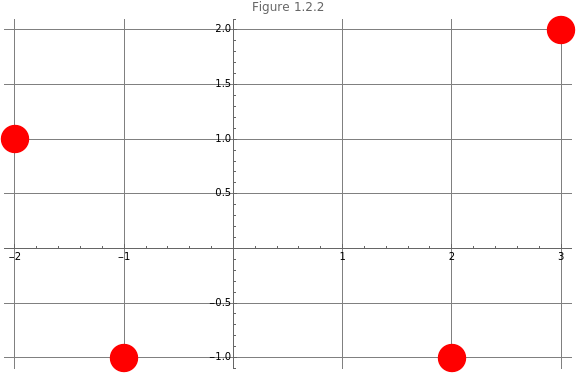
Below, we create four points, (3,2),(-2,1),(-1,-1) and (2,-1), one in each of the four named quadrants of the Cartesian plane. The quadrants are numbered using Roman numerals I, II, III, IV. The first quadrant is in the upper right corner where . The second quadrant is in the upper left corner where . The third quadrant is in the lower left corner with . Finally, the fourth quarter is in the lower right corner with . The four points are shown in Figure 1.2.2.
P
1
P
2
P
3
P
4
x>0,y>0
x<0,y>0
x<0,y<0
x>0,y<0
To start, though, we need to create the four points. This is done by creating list objects using the curly brace notation. The values of each of the and components of the points are listed inside the curly braces, separated by a comma. The equal symbol, =, is an assignment operator in the Wolfram Language. The assignment operator assign what is to its right, to the variable name on its left. The variable name is a user-chosen name. In the code cell below, the points are all assigned to the variable uppercase P, followed by an initial subscript counter value, through . The semi-colon after each creation of a list object and assignment to a variable, suppresses output to the screen.
x
y
1
4
In[]:=
(*Usinglistobjectstoholdthexandycoordinatevalues*)={3,2};={-2,1};={-1,-1};={2,-1};
P
1
P
2
P
3
P
4
We are now ready to plot the four points, through . The code for the generation of plots can, as mentioned before, be ignored until we properly introduce plotting later in the course.
P
1
P
4
In[]:=
(*UsingtheGraphicsfunctiontoplotthepoints*)Graphics[{PointSize[0.05],Red,Point[{,,,}]},AxesTrue,ImageSizeLarge,GridLines->Automatic,PlotLabel->"Figure 1.2.2"]
P
1
P
2
P
3
P
4
Out[]=
Definition 1.2.3 The Euclidean space refers to three-dimensional space. Any point in such space has three components, representing Cartesian coordinates. We follow the right-hand rule for the three mutually perpendicular , , and axes. Euclidean space is denoted as .
x
y
z
3
The point is shown in Figure 1.2.3.
P(2,3,1)
In[]:=
(*Plotapointin3-space*)Graphics3D[{PointSize[0.05],Red,Point[{2,3,1}]},AxesTrue,AxesLabel{"x","y","z"},ImageSizeLarge,PlotLabel->"Figure 1.2.3"]
Out[]=

Points may be located in hyperspace, with dimensions, denoted by .
n>3
n
Definition 1.2.3 The distance, , between two points, and , in the plane or in (hyper) space, both in and with , is defined in (1).
d
P(,,…,)
p
1
p
2
p
n
Q(,,…,)
q
1
q
2
q
n
n
n∈
d=
n
∑
i=1
2
(-)
p
1
q
1
(
1
)
Problem 1.2.1
Calculate the distance between points and in .
P(1,3,2,-1)
Q(2,2,1,4)
4
d(PQ)=+++=
2
(1-2)
2
(3-2)
2
(2-1)
2
(-1-4)
28
=27
(
2
)We verify our result with code using the EuclideanDistance function.
In[]:=
pointP={1,3,2,-1};pointQ={2,2,1,4};EuclideanDistance[pointP,pointQ]
Out[]=
2
7
1.3 Vectors
1.3 Vectors
1.3.1 Vectors in 2
1.3.1 Vectors in
2
There is another way to consider points in the Cartesian plane. We can imagine traveling from the origin at (0,0), along the and then the axis by a distance as indicated by the values of the tuple of a point. Starting at the origin and traveling to the point above, we travel units along the axis and then up, units, along the axis. Since this is a travel, we can demonstrate our path with an arrow, with its tail at the starting position and its head and the end position. Our two paths are shown in Figure 1.3.1.1.
P
o
x
y
(3,2)
3
x
2
y
To plot the two vector, we generate their starting and their end-positions as list objects assigned to an appropriate name.
In[]:=
(*Creatingthevectors*)tailX={0,0};headX={3,0};tailY=headX;headY={3,2};
The plot shows the two vectors in blue.
In[]:=
(*Plottingthetwovectors*)Graphics[{Blue,Thick,Arrow[{tailX,headX}],Arrow[{tailY,headY}]},AxesTrue,AxesLabel{"x axis","y axis"},PlotLabel"Figure 1.3.1.1",ImageSizeLarge,GridLines->Automatic]
Out[]=
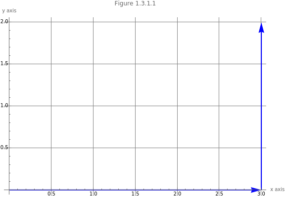
We have turned a point into a vector.
By definition, vectors of the same length and pointing in the same direction are the same vectors. These vectors are said to be equal. So, the two vectors depicted in Figure 1.3.1.3, are exactly the same vector.
Vector addition is the shown in (5) and is purely component-wise operation.
This is completely satisfying if we consider the explanation involving traveling along the axes as we had above.
Definition 1.3.1.2 A vector starting from the origin is a position vector.
To print the vector to the screen as a column vector, we use the MatrixForm function as pass the variable name v to it as parameter.
1.3.2 Vectors in space and hyperspace
1.3.2 Vectors in space and hyperspace
1.4 Length of a vector
1.4 Length of a vector
The ideas of the length of a vector and the direction of a vector are used in physics. These two descriptions completely describe a vector. Starting with length, also called the magnitude of a vector, we note that we can use the Pythagorean theorem to solve the problem of vector magnitudes.
Problem 1.4.1
The Norm function calculate the length of a vector. Vectors are created as list objects (using braces).
1.5 Unit vectors
1.5 Unit vectors
Problem 1.5.1
We create the vector as a list object and assign it to the variable v. The MatrixForm function prints the result as a vector.
1.6 Direction of a vector
1.6 Direction of a vector
We calculate the angle using (15).
Lastly, we have the fourth quadrant, shown in Figure 1.6.4.
We calculate the angle again using (15).
Definition 1.6.2 Two vectors are equal if they have the same magnitude and direction.
1.7 Vector arithmetic
1.7 Vector arithmetic
1.7.1 Vector addition
1.7.1 Vector addition
We have already seen vector addition in action, where we added the corresponding elements of two vectors to each other. We have to note here that vectors can only be added if they exist in the same space (with a similar number of components). We cannot add the two vectors in (16).
This addition is not defined.
The Wolfram Language will show us that it is so using the logical operator ==.
Vector addition is also associative, described in (19).
Again, since we inherit the property of commutativity from the real numbers (and each component is a real number), it is simple to prove this property for vectors in the same space.
Adding the zero vector to another vector returns that vector.
The == comparative operator confirms the equality.
Next, we consider scalar multiplication.
1.7.2 Scalar-vector multiplication
1.7.2 Scalar-vector multiplication
The equality in (22) follows.
1.7.3 Vector subtraction
1.7.3 Vector subtraction
Definition 1.7.3.1 Vector subtraction is then the addition of the negative (reverse) of a vector.
We can now do vector subtraction by adding this inverse.
The result is the zero vector (in the same space as the original vector).
1.8 Vector products
1.8 Vector products
1.8.1 Vector dot product
1.8.1 Vector dot product
The vector dot product or inner product is a simple concept. It can only be performed between vectors in the same space.
Definition1.8.1.1 The vector dot product multiplies corresponding elements of each vector and the resultant products are summed, as shown in (24).
We can use the Dot function to perform the dot product.
The period is short-hand notation for the dot product in the Wolfram Language.
1.8.2 Angle between vectors
1.8.2 Angle between vectors
We will use the magnitudes of these vectors as well as the law of cosines to construct an equation for the angle between vectors. Below, we see more about this law using Wolfram Alpha.
In[]:=
Law of Cosines
We use this law to write (25).
Definition 1.8.1.1 The (smallest) angle between two vectors is given in (27).
Problem 1.8.2.1
The solution is shown in (28).
We can verify this using the VectorAngle function.
Problem 1.8.2.2
Show that the two vectors generated as list objects in the code below are perpendicular.
Show that the two vectors generated as list objects in the code below are perpendicular.
We use the Dot function to calculate the dot product.
1.8.3 Orthogonal projections
1.8.3 Orthogonal projections
The dot product can be understood in terms of the orthogonal projection of one vector onto the other and the multiplication of the magnitude of this projection and the magnitude of the vector onto which we project.
We use (30) in the code cell below, where we start by generating the two vectors.
1.9 Vector cross product
1.9 Vector cross product
The cross product is easily calculated from the determinant (chapter 4) where we create a matrix (chapter 2) with the first row being the elementary unit vectors and the subsequent rows are the two vectors.
For now, we can use the Cross function to show us the equation for the cross product of two 3-space vectors.
Note that the result is a vector in 3-space.
The reason for this will be clear when we consider the angle between vectors. It should be clear, though, that parallel vector seen as position vectors are coincident and we cannot define a vector that is uniquely orthogonal to this.