2 | Lines and planes
2 | Lines and planes
This chapter of Multivariable Calculus by Dr JH Klopper is licensed under an Attribution-NonCommercial-NoDerivatives 4.0 International Licence available at THE CREATIVE COMMONS .
2.1 Introduction
2.1 Introduction
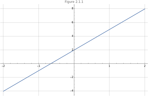
We are all familiar with lines in created by single variable functions such as , plotted in Figure 2.1.1. In multivariable calculus we are also familiar with planes such as , plotted in Figure 2.1.2.
2
y=3x+2
z=2x+y
In[]:=
Plot[3x+2,{x,-2,2},PlotLabel"Figure 2.1.1",ImageSizeLarge,GridLines->Automatic]
Out[]=
In[]:=
Plot3D[2x+y,{x,-2,2},{y,-2,2},MeshNone,PlotLabel"Figure 2.1.2",ImageSizeLarge]
Out[]=

We now extend our understanding of these concepts in terms of vectors.
2.2 Lines in 2
2.2 Lines in
2
As mentioned, lines in are expressed as a single variable equation shown in (1).
2
y=f(x)=mx+c
(
1
)Here, is the slope and is the intercept (when ).
m
c
y
x=0
We can parametrize this line. This gives it a direction as well as a given start and a given finish value for the parameter. This means that we have a start and an end-point of a segment of the line. For (1), using a parameter, , we get (2).
t
x(t)=ty(t)=mt+c
(
2
)This allows us to express the line as a vector, (3), where we use angled bracket notation.
r(x(t),y(t)=〈t,mt+c〉
(
3
)
Problem 2.2.1
Express the line in (4) in parametric form. This is the line we plotted above.
y=3x+2
(
4
)Solution
We choose a simple parametrization in (5).
x(t)=ty(t)=3t+2
(
5
)The ParametricPlot function allows us to enter the vector and the start and end parameter value. This is shown in Figure 2.2.1.
In[]:=
ParametricPlot[{t,3t+2},{t,0,4},PlotRange{0,15},AspectRatio1,PlotLabel"Figure 2.2.1",ImageSizeLarge,GridLines->Automatic]
Out[]=
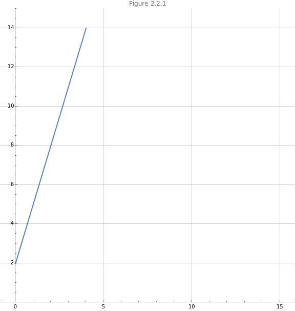
We now see a segment of the line. If we want to recreate the whole line, we need to let the domain of our parameter be .
t∈(-∞,∞)
2.3 Plane curves
2.3 Plane curves
It is not only straight lines that can be parametrized. We can do the same with curves.
Problem 2.3.1
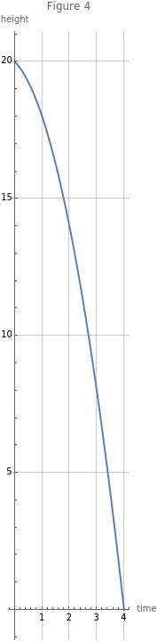
Parametrize and plot the function in (6) for the parameter domain , indicating the height of a falling object over time.
t∈[0,3]
y=--x+20
2
x
(
6
)We introduce a simple parametrization, . This results in (7) and we plot the plane curve using the ParametricPlot function in Figure 2.3.1.
x=t
r(x(t),y(t))=〈t,--t+20〉,0≤t≤4
2
t
(
7
)In[]:=
ParametricPlot[{t,--t+20},{t,0,4},AxesLabel{"time","height"},PlotLabel"Figure 2.3.1",ImageSizeLarge,GridLines->Automatic]
2
t
Out[]=
Problem 2.3.2
Plot the parametric curve in (8).
Figure 2.3.2 is created using the ParametrixPlot function. The result is a curve in the plane that we do not associate with a function.
Problem 2.3.3
Consider the plane curve in (10).
Plot the curve of the function.
A plot of this is shown in Figure 2.3.3.
In Figure 2.3.4, we use the Manipulate function to show the evolution of the plane curve over the domain of the parameter, including its direction of change.
Using the Manipulate function to visualize the parametrization
Problem 2.3.4
Parametrize and plot the function in (12).
We can rewrite the function of the plane curve, (13).
In Figure 2.3.5, we plot the parametric equation.
In Figure 2.3.7, we double the parameter, but halve the domain.
Problem 2.4.1
Problem 2.4.2
Do the two line in (22) intersect in 3-space?
Solution
It does not look as if they intersect. To confirm this we start by looking if they are parallel. If so, their direction vectors should be scalar multiples of each other, (23).
Problem 2.4.3
We see the result in Figure 2.4.3.
They intersect indeed, but not at the same time. We see the with the Manipulate function in Figure 2.4.4.
The point of intersection is therefor as in (29).
Problem 2.4.4
From the parametric equations, we have two directional vectors shown in (30).
We can use the dot product equation to calculate the angle, shown in (31).
We get a numeric approximation for this angle in radians using the N function.
Problem 2.4.5
2.5 Normal vectors
2.5 Normal vectors
Definition2.5.1 A normal vector is a vector that is orthogonal (perpendicular) to a plane.
2.6 Equations of planes
2.6 Equations of planes
2.6.1 Equation of a plane given a normal to the plane and a point in the plane
2.6.1 Equation of a plane given a normal to the plane and a point in the plane
Problem 2.6.1.1
Find the equation of a plane with a normal to the plane and a point on the plane given in (38).
2.6.2 Equation of a plane given three points in the plane
2.6.2 Equation of a plane given three points in the plane
Problem 2.6.2.1
Find the equation of the plane given three points in (40).
2.6.3 Equation of a plane given a point and a line in the plane
2.6.3 Equation of a plane given a point and a line in the plane
Problem 2.6.3.1
Calculate the equation of the plane that contains the point and the line in (42).
With two points, we create another vector, this time, in the plane, (44).
The cross product gives us a normal and we use the same steps as in the previous problem.
The solution is shown in (45).
2.6.4 Equation of a plane given two points in the plane and a perpendicular plane
2.6.4 Equation of a plane given two points in the plane and a perpendicular plane
Problem 2.6.4.1
Find the equation of a plane given two points on the plane and another plane perpendicular to it, (46).
We can extract the normal to the perpendicular plane. This is shown in (47). Since it is orthogonal to this plane, it is parallel to the plane for which we seek an equation.
We can create another vector in our plane from the two given points, shown in (48).
Now we follow these steps:
1. Cross product between normal vector (to perpendicular plane) and vector in the plane normal to the desired plane
2. Cross product between this normal vector and an arbitrary vector in the desired plane equation of the desired plane
1. Cross product between normal vector (to perpendicular plane) and vector in the plane normal to the desired plane
2. Cross product between this normal vector and an arbitrary vector in the desired plane equation of the desired plane
The solution is in (49).
2.7 Angles between planes
2.7 Angles between planes
Problem 2.7.1
Calculate the angle between the planes in (50).
Solution
The normals to these planes are shown in (51).
These vectors are not scalar multiples of each other. They are therefor not parallel. Below, we look at the dot product.
The numerical approximation is confirmed using the N function.
2.8 Angle between a line and a plane
2.8 Angle between a line and a plane
2.9 Line of intersection of planes
2.9 Line of intersection of planes
The line of intersection between two planes has a direction vector. This vector is orthogonal to the plane made by the two normals of the planes.
Problem 2.9.1
Calculate the direction vector of a line that is the intersection of the two planes in (54).
We can plot the two planes, using the ContourPlot3D function, shown in Figure 15.
The two normals and their cross product is shown below.
We solve these two equations for two unknowns using the RowReduce function on the augmented matrix.
2.10 Distance between a point and a plane
2.10 Distance between a point and a plane
Consider the image below.
Substituting, we get the equation for the distance between a point and a plane, shown in (59).
So, to solve for this problem, we need the equation of the plane and the point coordinate.
Problem 2.10.1
Calculate the distance between the point and plane in (60).
This is easily solved in (61).
2.11 Distance between parallel planes
2.11 Distance between parallel planes
This follows from the distance between a point and a plane. We only require an arbitrary point on the second plane.
Problem 2.11.1
Calculate the distance between the two planes in (62).