3 | Spheres, Cylinders, and Surfaces
3 | Spheres, Cylinders, and Surfaces
This chapter of Multivariable Calculus by Dr JH Klopper is licensed under an Attribution-NonCommercial-NoDerivatives 4.0 International Licence available at THE CREATIVE COMMONS .
3.1 Introduction
3.1 Introduction
In this notebook we take our first look at spheres, cylinders, and surfaces in . This is similar to the journey we took when we first learned about lines associated with single-variable functions. We all know that is a parabola and is a straight line. The same can be said for functions of two variables, , where we express three variables, , , and .
3
y=
2
x
y=mx+c
z=f(x,y)
x
y
z
Let’s get familiar with these surfaces, which we will do by way of a set of example problems. We start off with spheres and cylinders, which are examples of second-degree equations in , before looking at quadratic surfaces.
3
3.2 Spheres
3.2 Spheres
Definition 3.2.1 A sphere, , is the set of all points which are a fixed distance, , called the radius, away from a fixed point (,,), shown in (1).
S
(x,y,z)∈
3
r
P
0
x
0
y
0
z
o
S=(x,y,z)++=
2
(x-)
x
0
2
(y-)
y
0
2
(z-)
z
0
2
r
(
1
)It is also defined in terms of vectors, and =(,,), shown in (2).
x=(x,y,z)
x
0
x
0
y
0
z
0
S={x:||x-||=r}
x
0
(
2
)As mentioned, spheres are second-degree equations in .
3
Problem 3.2.1
Write the equation in in the from shown in (1).
2+2+2-6x-4y+2z=1
2
x
2
y
2
z
3
We have to transform the equation into the form in (1). To do this we group the terms and complete the squares, as shown in (3).
2(-3x)+2(-2y)+2(+z)=1(-3x)+(-2y)+(+z)=-3x++-2y+++z+=++1++=
2
x
2
y
2
z
2
x
2
y
2
z
1
2
2
x
2
-
3
2
2
y
2
-
2
2
2
z
2
1
2
1
2
9
4
2
x-
3
2
2
(y-1)
2
z+
1
2
2
2
(
3
)The center of the sphere is therefor and the radius .
C,1,-
3
2
1
2
r=2
3.3 Cylinders
3.3 Cylinders
Cylinders are also second-degree equations in .
3
Definition 3.3.1 A cylinder is a surface along an axis in .
3
The equation for the cylinder only contains two variables and the cylinder extends along the axis of the missing variable (from , , and ). When given the equation, we must be informed that it is an equation in or else it will appear as a simple equation in .
x
y
z
3
2
Problem 3.3.1
Plot the equation . Note then that this is not .
z=f(x,y)=4-
2
x
z=f(x)=4-
2
x
We plot this cylinder in Figure 3.3.1 using the ContourPlot3D function.
In[]:=
ContourPlot3D[z4-,{x,-3,3},{y,-5,5},{z,-3,5},MeshNone,BoundaryStyleNone,AxesLabel{"x axis","y axis","z-axis"},PerformanceGoal"Quality",PlotLabel"Figure 3.3.1",ImageSizeLarge]
2
x
Out[]=

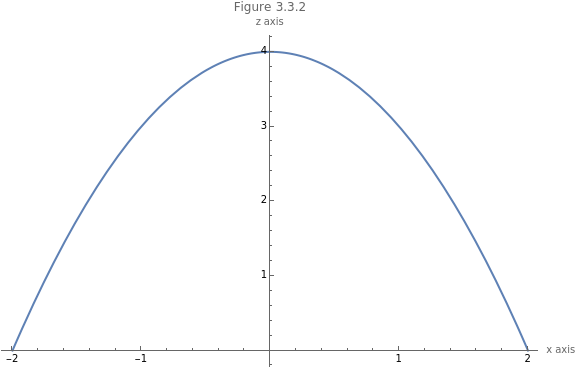
Note how the cylinder extends along the (missing) axis. No matter where along the axis we make a sagittal cut (a constant value for that is parallel to the plane), we get the same shape along the and axes. We see what the cylinder is going to look like in the plane by setting using the Plot function in Figure 3.3.2.
y
y
y
xz
x
z
xz
z=4-
2
x
In[]:=
Plot[4-,{x,-2,2},AxesLabel{"x axis","z axis"},PlotLabel"Figure 3.3.2",ImageSizeLarge]
2
x
Out[]=
Problem 3.3.2
Plot the equation in .
9+4=36
2
x
2
y
3
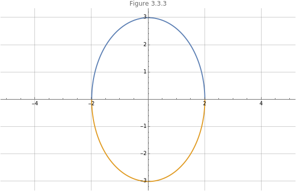
This cylinder will extend along the axis. This time around, let’s start by looking at the plane, where . In Figure 3.3.3, we have solved for .
z
xy
z=0
y
In[]:=
Plot,-,{x,-5,5},PlotLabel"Figure 3.3.3",GridLines->Automatic,ImageSizeLarge
36-9
2
x
4
36-9
2
x
4
Out[]=
Definition 3.3.2 The standard form of an ellipse as a cylinder is as shown in (4).
2
x
2
a
2
y
2
b
(
4
)We transform the equation in the problem above into the standard form for an ellipse in (5).
9+4
2
x
2
y
36
2
x
2
2
2
y
2
3
2
6
(
5
)This ellipse is extended along the axis, and shown in Figure 3.3.4 using the ContourPlot3D function.
z
In[]:=
ContourPlot3D[9+436,{x,-3,3},{y,-5,5},{z,-3,5},MeshNone,BoundaryStyleNone,ContourStyleDirective[Opacity[0.8]],AxesLabel{"x axis","y axis","z-axis"},PerformanceGoal"Quality",PlotLabel"Figure 3.3.4",ImageSizeLarge]
2
x
2
y
Out[]=

Problem 3.3.3
We rewrite the equation in (6).
The cylinder is shown in Figure 3.3.6.
(Unfortunately, the asymptotic plane is drawn as well.)
3.4 Surfaces
3.4 Surfaces
Surfaces contain all three variables, with the plot changing along the third axis as opposed to being constant as with a cylinder. They are termed quadratic surfaces.
3.4.1 Ellipsoids
3.4.1 Ellipsoids
Definition 3.4.1.1 An ellipsoid is a quadratic surface with a standard form equation defined in (7).
Problem 3.4.1.1
We put this in standard form in (8).
The solution is shown in Figure 3.4.1.1.
3.4.2 Hyperboloid of one sheet
3.4.2 Hyperboloid of one sheet
Any of the terms in the standard form of a quadratic surface can be the negative.
Definition 3.4.2.1 A hyperboloid of one sheet is a quadratic surface with a standard form equation defined in (9).
The negative term is the axis of travel.
Problem 3.4.2.1
Solution
3.4.3 Hyperboloid of two sheets
3.4.3 Hyperboloid of two sheets
Definition 3.4.3.1 A hyperboloid of two sheets is a quadratic surface with a standard form equation defined in (10).
In this quadratic surface, we have two negative terms. The surface is directed along the axis with the positive term.
Problem 3.4.3.1
We have to transform the equation as shown in (11). The right -hand side must be positive.
The solution is shown in Figure 3.4.3.1.
3.4.4 Elliptic cones
3.4.4 Elliptic cones
Definition 3.4.4.1 An elliptic cone is a quadratic surface with a standard form equation defined in (12).
Problem 3.4.4.1
We transform this in (13) so as to recognize the surface.
The solution is shown in Figure 3.4.4.1.
3.4.5 Elliptic paraboloids
3.4.5 Elliptic paraboloids
Definition 3.4.5.1 An elliptic paraboloid is a quadratic surface with a standard form equation defined in (14).
Problem 3.4.5.1
We transform the the equation in (15) so as to recognize the surface.
The solution is shown in Figure 3.4.5.1.
3.4.6 Hyperbolic paraboloids
3.4.6 Hyperbolic paraboloids
Definition 3.4.6.1 A hyperbolic paraboloid is a quadratic surface with a standard form equation defined in (16).
The graph is a saddle.
Problem 3.4.6.1
We transform this in (17), so as to recognize the surface.
The solution is shown in Figure 3.4.6.1.