4 | Coordinate systems
4 | Coordinate systems
This chapter of Multivariable Calculus by Dr JH Klopper is licensed under an Attribution-NonCommercial-NoDerivatives 4.0 International Licence available at THE CREATIVE COMMONS .
4.1 Introduction
4.1 Introduction
We are all familiar with the rectangular coordinate system. In two-dimensional space, we have the Cartesian plane with standard unit vectors and along the and axes. In three-dimensional space, we add a third (right-handed) axis, perpendicular to the plane, resulting in Cartesian space. This is the axis with standard unit vector . An area or volume can be expressed in term of , , and components, with functions and bounds defined in terms of these variables.
i
j
x
y
xy
z
k
x
y
z
The rectangular coordinate system is not always the best coordinate system to use when solving problems, though. In this notebook, we look at transformation to two other coordinate systems (cylindrical and spherical coordinate systems) and how that relates to spheres, cylinders, and surfaces.
4.2 Rectangular coordinates
4.2 Rectangular coordinates
In , we express any point in terms of a 3-tuple, , where . In Figure 4.2.1, we plot the point .
3
P
(x,y,z)
x,y,z∈
P(
2
,-2
,4)In[]:=
Graphics3D[PointSize[0.05],Red,Point[
2
,-2
,4],AxesTrue,PlotRange{{1,2},{-1,-2},{3,5}},AxesLabel{"x axis","y axis","z axis"},PlotLabel"Figure 4.2.1",ImageSizeLarge]Out[]=

4.3 Rectangular and cylindrical coordinates
4.3 Rectangular and cylindrical coordinates
Definition 4.3.1 The cylindrical coordinate system expresses points in space according the the distance, , from to origin to the projection of the point on the plane, and the angle, , from the positive axis to the line from the origin to this projection, anti-clockwise from the positive -axis on the interval and clockwise from the positive -axis on the interval . The height of the point along the axis remains.
r
xy
θ
x
x
[0,π]
x
(-π,0)
z
In the image below, we see a point in -space, similar to the one we used in Figure 4.2.1. Its projection down onto the plane is a distance from the origin (therefor ) and makes an angle of with the positive axis as described above. It is at a height . These are the components of a point in cylindrical coordinates, .
P(x,y,z)
3
xy
r
r≥0
θ
x
z
P(r,θ,z)
In[]:=
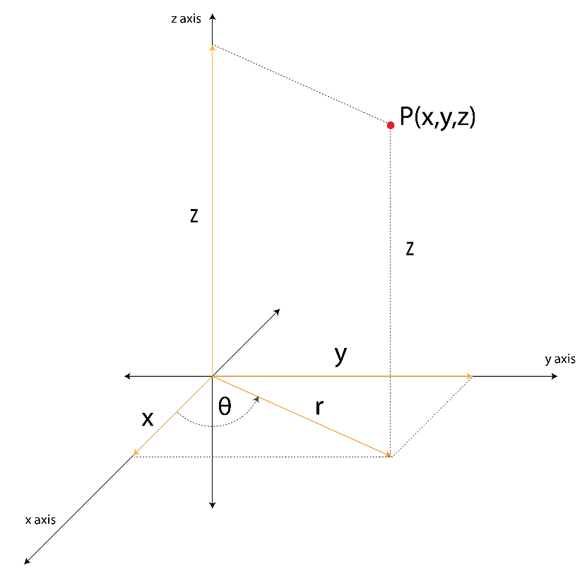
To transform this point from components to cylindrical components is a fairly simple procedure and follows from the geometry in the image above. The equations of transformation (from cylindrical to rectangular coordinates) are shown in (1).
(x,y,z)
(r,θ,z)
r=+θ=arctanz=z
2
x
2
y
y
x
(
1
)The CoordinateTransform function allows us to verify the results. The arguments are self-explanatory.
In[]:=
CoordinateTransform["Cartesian""Cylindrical",{x,y,z}]
Out[]=
+,ArcTan[x,y],z
2
x
2
y
A list object containing the three expressions for ,θ, and respectively are returned.
2
r
z
Note that the ArcTan function parameters list the denominator first and the the numerator .
x
y
The equations for transformation from cylindrical coordinates to rectangular coordinates are shown in (2) and are again easily deduced from the image above.
(r,θ,z)
(x,y,z)
cos(θ)=x=rcos(θ)sin(θ)=y=rsin(θ)z=z
x
r
y
r
(
2
)As before, the CoordinateTransform function allows us to verify the results.
In[]:=
CoordinateTransform["Cylindrical""Cartesian",{r,θ,z}]
Out[]=
{rCos[θ],rSin[θ],z}
These transformations follow from the Pythagorean Theorem and trigonometry.
Problem 4.3.1 Transform the point from rectangular to cylindrical coordinates.
P(
2
,-2
,4)The solution follows in (3) from (2).
2
r
2
(
2
)2
(-
2
)π
4
π
4
(
3
)We use the CoordinateTransform function to verify the result.
In[]:=
CoordinateTransform["Cartesian"->"Cylindrical",
2
,-2
,4]Out[]=
2,-,4
π
4
We can plot this point (and a vector to it) as shown in Figure 4.2.2. Note that the radius is always positive. We express an angle with the positive axis going counter-clockwise, but as soon as the angle is more than radians, we express it as a negative angle going clockwise from the positive axis.
0≤θ≤π
x
π
x
In[]:=
Graphics3D[PointSize[0.05],Red,Point[
2
,-2
,4],Orange,Thick,Arrow[{0,0,0},2
,-2
,4],AxesTrue,AxesLabel{"x axis","y axis","z axis"},PlotLabel"Figure 4.3.1",ImageSizeLarge]Out[]=

This is done using the equations in (2) and is shown in (4).
We use the CoordinateTransform function to verify the result.
4.4 Rectangular and spherical coordinates
4.4 Rectangular and spherical coordinates
We use the equations in (5) for transformation from spherical to rectangular coordinates and the equations in (6) for transformation from spherical to rectangular coordinates.
The ToSphericalCoordinates function is used to transform a point in rectangular coordinates to a point in spherical coordinates.
The FromSphericalCoordinates function is used to transform a point in spherical coordinates to a point in rectangular coordinates.
The CoordinateTransform function can also be used.
The point is shown in Figure 4.4.1.
This is done using the equations in (6).
We verify the result below using the FromSphericalCoordinates function.
4.5 Cylindrical and spherical coordinates
4.5 Cylindrical and spherical coordinates
In (7), we list the transformations from rectangular to cylindrical coordinates and from cylindrical back to rectangular coordinates. We then use the equations for the transformation from spherical coordinates to rectangular coordinates and substitute where required.
This is done in (8).
The CoordinateTransform function confirms the results.
This is done in (10).
We confirm the trigonometric calculations using the Wolfram Language.
The CoordinateTransform function is used to verify the solution.
4.6 Identifying spheres, cylinders, and surfaces for equations
4.6 Identifying spheres, cylinders, and surfaces for equations
Recognizing surface from given equations is important in multivariable calculus. It is particular interest when we start to consider regions and surfaces as bounds for double and triple integrals.
The equations require manipulation using the transformation equations above.
The SphericalPlot3D function is used to visualize the solution in Figure 4.6.2. Note the order of the angles, though.
This is done using transformation in (18).
This is done using transformation in (20).
This is done using transformations in (22).
This is done using transformations in (24).
This is done using transformations in (26).
Problem 4.6.9 Express an equation for (27) in 3-space.
This is done using transformation in (28).
Problem 4.6.10 Express an equation for (29) in 3-space.
This is done using transformation in (30).