5 | Plane Curves and Parametric Equations
5 | Plane Curves and Parametric Equations
This chapter of Multivariable Calculus by Dr JH Klopper is licensed under an Attribution-NonCommercial-NoDerivatives 4.0 International Licence available at THE CREATIVE COMMONS .
5.1 Introduction
5.1 Introduction
Parametric equations provide a way to describe a curve by defining its -coordinate and -coordinate as functions of a third variable, typically . This can be useful for modeling motion, or for describing curves that are difficult to define using Cartesian equations of the form .
x
y
t
y=f(x)
In this chapter, we will learn how to differentiate and integrate parametric functions. This will allow us to find the slope, velocity, and acceleration of a moving objects, as well as the area enclosed by a parametric curve.
5.2 Parametric functions
5.2 Parametric functions
Definition 5.2.1 A parametric function defines a curve of a function by expressing its -coordinate and -coordinate as functions of a third variable, typically . A parametric function is a pair of equations of the form and .
y=f(x)
x
y
t
x=x(t)
y=y(t)
5.2.1 Generating and plotting parametric curves of a single variable function
5.2.1 Generating and plotting parametric curves of a single variable function
Consider the polynomial function in (1) on the closed interval , where .
[0,4]
x,y∈
y=-+4,x∈[0,4]
2
(x-2)
(
1
)In Figure 5.2.1.1 we plot this single variable function.
In[]:=
Plot[-+4,{x,0,4},PlotLabel"Figure 5.2.1.1",AxesLabel{"x axis","y axis"},GridLines->Automatic,ImageSizeLarge]
2
(x-2)
Out[]=
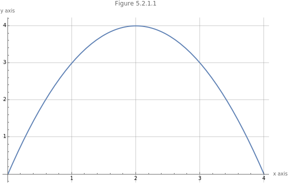
We can determine any value of the dependent variable given a value for the independent variable . This gives us a continuous curve in the plane for the specified domain .
y
x
x∈[0,4]
The curve can also be viewed as a path, starting at a point on the curve and moving along the curve given a parameter. We often use time as a parameter and hence the variable . This process is termed parametrization of a curve. Here, both the dependent variable, , and the independent variable, , become functions of the parameter, .
t
y
x
t
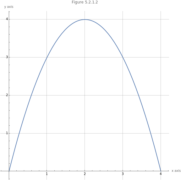
In a simple parametrization of the function in (1), we might have by simple assignment and substitution that and therefor . Each point on the curve is now a 2-tuple ). We get the same curve for the interval of the parameter since . We plot this curve using the ParametricPlot function in Figure 5.2.1.2.
x(t)=t
y(t)=-+4
2
(t-2)
(x(t),y(t)
t∈[0,4]
x(t)=t
In[]:=
ParametricPlot[{t,-+4},{t,0,4},PlotLabel"Figure 5.2.1.2",AxesLabel{"x axis","y axis"},GridLines->Automatic,ImageSize->Large]
2
(t-2)
Out[]=
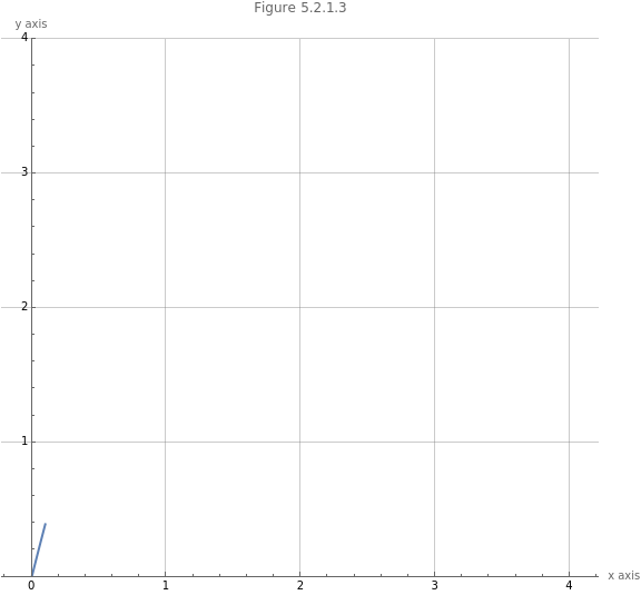
Using the Manipulate function in Figure 5.2.1.3, we can see how the parameter progresses the curve. Note that we use the placeholder variable in the plot below.
t
s
In[]:=
Manipulate[ParametricPlot[{s,-+4},{s,0,t},AxesLabel{"x axis","y axis"},PlotRange{0,4},PlotLabel"Figure 5.2.1.3",GridLines->Automatic,ImageSizeLarge,ImageSizeLarge],{{t,0.1,"The time parameter t"},0.1,4}]
2
(s-2)
Out[]=


There is not a single parametrization of a curve. By letting in (1), we than have that . Since we have that to consider the interval in terms of . Here we have that because implies . The result is shown in Figure 5.2.1.4.
x(t)=2t
y(t)=-+4=-4+8t
2
(2t-2)
2
t
x∈[0,4]
t
t∈[0,2]
x(t)=2t
t=x
1
2
In[]:=
ParametricPlot[{2t,-+4},{t,0,2},PlotLabel"Figure 5.2.1.4",AxesLabel{"x axis","y axis"},GridLines->Automatic,ImageSizeLarge]
2
(2t-2)
Out[]=

Problem 5.2.1.1 Plot the parametric function in (2).
5.2.2 Eliminating the parameter
5.2.2 Eliminating the parameter
When a single variable function is presented as a parametric function, it can be of benefit to eliminate the parameter using substitution and then using prior knowledge of single variable functions to identify the curve of the function.
Problem 5.2.2.1 Eliminate the parameter of the parametric equation in (5).
Problem 5.2.2.2 Eliminate the parameter from the parametric equation in (7).
The solution is written in (8).
To verify that this is correct, we plot the original parametric function and animate it on the interval for the parameter in Figure 5.2.2.2.
Problem 5.2.2.3 Eliminate the parameter and plot the curve of parametric equation in (9).
To solve this problem, we make use of a trigonometric identity for the solution shown in (10).
5.3 Derivatives of parametric equations
5.3 Derivatives of parametric equations
5.3.1 First derivatives of parametric equations
5.3.1 First derivatives of parametric equations
Consider the function in (11).
A parameterization of (11) is shown in (12).
We can differentiate both function in (12), which is shown in (13) below.
The first derivate of the function in (11), is shown in (14).
Note how the first derivate in (14) can be written as in (15).
This is not a coincidence or a special case. Indeed, we can use the chain rule to derive a method for taking the derivate of a parametrized function.
Theorem 5.3.1.1 The derivative of a parametrized function is as denoted in (15).
Substitution and using Leibniz notation using (16) and (17) yields (15).
Problem 5.3.1.1 Calculate the first derivative of the parametric functions in (18).
The derivative of the first parametric equation in (18) is calculated in (19).
The derivative is calculated using the D function.
The Solve function can be used to calculate the roots.
Problem 5.3.1.2 Calculate the first derivative of the parametric functions in (22)
The derivative of the second parametric equation is calculated in (23).
The result is verified using code below.
The parametric function is plotted in Figure 5.3.1.3.
We calculate both derivatives using the D function below.
In (25), we substitute the results from the code and calculate the first derivative.
5.3.2 Vertical and horizontal tangent lines
5.3.2 Vertical and horizontal tangent lines
Problem 5.3.2.1 Calculate the rectangular coordinates of the point on the parametric equation shown in (28), where the derivative of the equation is undefined.
The graph of the equation is shown in Figure 5.3.2.1.
5.3.3 Second derivatives of parametric equations
5.3.3 Second derivatives of parametric equations
Problem 5.3.3.1 Calculate the second derivative for the plane curve defined by the parametric equations in (30).
We have already calculated the first derivative. It is calculated again using code below.
5.4 Integrals of parametric curves
5.4 Integrals of parametric curves
5.4.1 The integral of a parametric equation
5.4.1 The integral of a parametric equation
Simple algebra (which is permissible here and done without motivation) yields (32).
Substitution into (31) yields the equation for the integral of a parametric function, shown in (33).
We can achieve the same equation using Riemann sums.
Problem 5.4.1.1 Calculate the area under curve of the cycloid defined by the parametric equations in (34).
Solution 5.4.1.1 The curve of the parametric equation in (34) is shown in Figure 5.4.1.1.
We see the substitution in (35).
We also use the code below to verify the result.
Problem 5.4.1.2 Calculate the area under the curve of hypocycloid defined in (36).
The curve of the equation in (35) is shown in Figure 5.4.1.2.
The problem is written in (37).
We use the Simplify function to simply the integrand.
The integral is calculated below.
5.4.2 Arc length of a parametric equation
5.4.2 Arc length of a parametric equation
Our aim is to derive a function to compute the length of a curve on a plane, called the arc length.
It does not cross itself. If it does so, it must be at a finite number of points.
Any small segment is then as described in (40).
In (42) we use the Pythagorean Theorem for this length.
We substitute this into (42) and simplify as shown in (44).
Problem 5.4.2.1 Calculate the arc length of the semi-circle defined by the parametric equation in (46).
The problem is visualized in Figure 5.4.2.1.
The derivatives of the parametric component functions are calculated below.
The function for calculating the arc length of a parametric curve is used in the code calculation below.
Problem 5.4.2.2 Calculate the arc length of the parametric equation in (47).
The problem is visualized in Figure 5.4.2.2.
We can calculate the square of the first derivatives below.
Now, we take the derivative of square root of the sum of these terms over the required interval.
Problem 5.4.2.3 Calculate the arc length of the parametric equation defined in (48).
The problem is visualized in Figure 5.4.3.2.
The derivates and the integral are calculated below.
5.4.3 Surface area generated by a parametric equation
5.4.3 Surface area generated by a parametric equation
Definition 5.4.3.1 A simple closed curve is the curve of a parametric equation when the curve does not cross itself and the point on the curve at the bounds of the parameter coincide.
For clockwise rotation (interchange of beginning and end value of the parameter), the sign changes.
Simple substitution yields (49).
Problem 5.4.3.1 Calculate the area of an ellipse given in (52).
We can use parametrization with the following equations, shown in (53).
Below, we confirm our result using the Wolfram Language. We have the area of an ellipse.
5.5. Appendix
5.5. Appendix
5.5.1 Mean value theorem
5.5.1 Mean value theorem
Consider the third-order polynomial in (55).
We can calculate the value of the secant line between these two points as shown in (59).
We plot the interval and the secant line in Figure 5.5.1.2.
On our interval we note the solution in (60).
We use point slope form to solve for the equation at the point and add the slope on a short interval in (61).
Figure 5.5.1.3 visualizes the result.