6 | Vector-valued Functions
6 | Vector-valued Functions
This chapter of Multivariable Calculus by Dr JH Klopper is licensed under an Attribution-NonCommercial-NoDerivatives 4.0 International Licence available at THE CREATIVE COMMONS .
6.1 Introduction
6.1 Introduction
In this chapter we explore the concept of vector-valued functions, an extension of the familiar real-valued functions. These functions include vectors as opposed to single or multiple variables. This shift to vectors allows us to describe not just magnitude but also direction, encapsulating a more comprehensive picture of various phenomena.
6.2 Vector functions
6.2 Vector functions
In this notebook, we view vector functions as parametrizations of single variable functions. We see an example of such a vector function, , of three variables in (1), where we use the parameter .
α
t
α(x,y,z)=(f(t),y(t),z(t))
(
1
)Definition 6.2.1 A vector function is a mapping from its domain, , to its range, . Here is a variable and for every in , we have a single vector , where . We use the variable as vector function most commonly referring to time.
D⊂
R⊂
3
t∈
t
D
α=r(t)
α∈
3
t
This allows us to create a vector function, shown in (2), that traces a curve in 3-space with a domain .
t
r(t)=x+y+z
i
j
k
(
2
)The equation in (2) is called a component function. There are three components in the vector function in (2), . We can also write the vector function as in (3), using angled bracket notation.
x,y,z
i
i
k
r(t)=〈f(t),g(t),h(t)〉
(
3
)The domain of the parameter, , is defined on an interval. This is either evident or must be derived from looking at the intervals defined for the components of the vector function.
t
Problem 6.2.1 Express the domain for the variable in the vector function in (4), containing three components.
t
r(t)=,log(t)
t
,1
t-1
(
4
)This is done by combining the domains of the parameter for each component and is shown in (5).
x:0≤t≤∞y:t≠1z:t>0t∈(0,1)⋃(1,∞)
(
5
)It is also possible to recreate the original single variable function, given a vector function.
Problem 6.2.2 Express an equation for the vector function in (6).
y=f(x)
r(t)=
t
,4-t,t∈[0,∞)(
6
)This is done by substitution and shown in (7).
x==ty=4-ty=4-
t
2
x
2
x
(
7
)This is the half of a parabola extending to the axis, to the right of and intersecting the axis at . The reason why we do not consider the rest of the parabola towards (although is defined on the interval ), is because of the domain of the parameter, . We note that is only defined for .
-y
x=0
y
4
-∞
y=4-
2
x
(-∞,∞
t
x=
t
t≥0
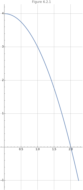
We can plot the vector function in (6) using the ParametricPlot function and this is shown in Figure 6.2.1.
In[]:=
ParametricPlot[
t
,4-t,{t,0,5},PlotLabel"Figure 6.2.1",GridLines->Automatic,ImageSizeLarge]Out[]=
Problem 6.2.3 Express an equation of the form for the vector function in (8).
y=f(x)
r(t)=〈t+1,-2〉,-2≤t≤2
2
t
(
8
)The solution follows substitution (9).
x=t+1t=x-1y=-2=-2x+1-2=-2x-1
2
(x-1)
2
x
2
x
(
9
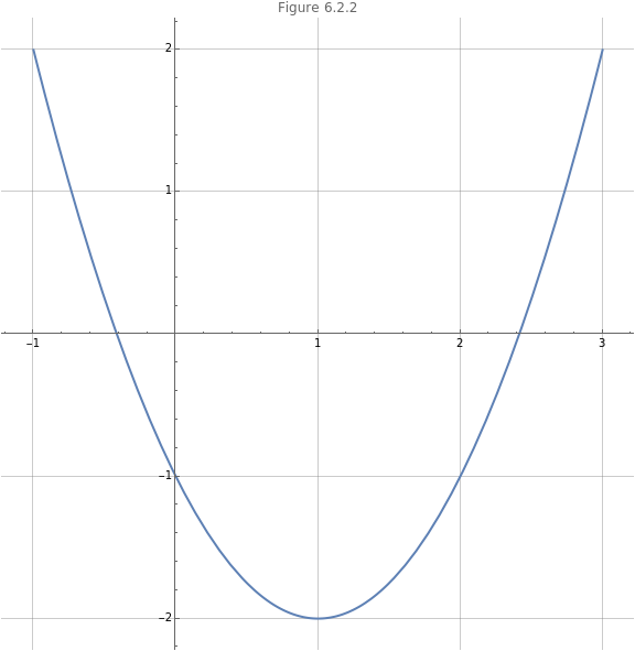
)This is a parabola shifted down and to the right, shown in Figure 6.2.2. Note that .
2
1
t∈(-∞,∞)
In[]:=
ParametricPlot[{t+1,-2},{t,-2,2},PlotLabel"Figure 6.2.2",GridLines->Automatic,ImageSizeLarge]
2
t
Out[]=
Problem 6.2.4 Express an equation for the vector function in (10).
r(t)=4cos(t)-3sin(t),t∈[0,2π]
i
j
(
10
)We solve for the trigonometric functions of and use a trigonometric identity in (11).
t
cos(t)=,sin(t)=-(t)+(t)=+=1,=
x
4
y
3
2
cos
2
sin
2
x
4
2
y
3
2
-
y
3
2
y
3
(
11
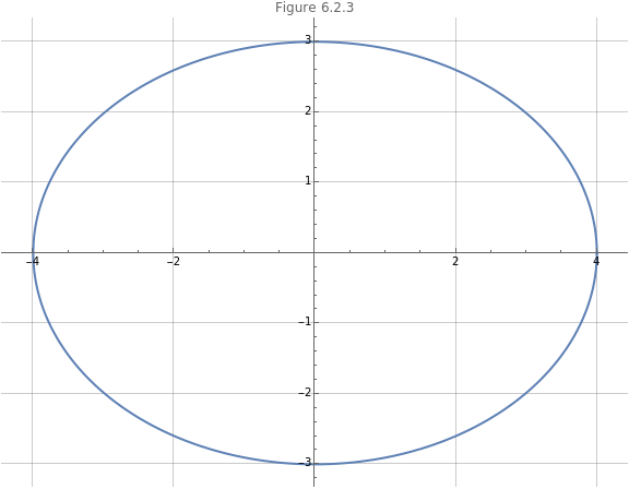
)This is the equation of an ellipse, shown in Figure 6.2.3.
In[]:=
ParametricPlot[{4Cos[t],-3Sin[t]},{t,0,2π},PlotLabel"Figure 6.2.3",GridLines->Automatic,ImageSizeLarge]
Out[]=
Problem 6.2.5 Determine the physical representation of the vector function in (12).
We recognize the parametric equation of a line in (13).
Problem 6.2.6 Express an equation for the vector function in (14).
This is done by substitution and the use of a trigonometric identity in (15).
This is a cylinder on which the curve exists. We see this surface in Figure 6.2.5.
The actual parametric curve is shown in Figure 6.2.6.
6.3 Derivatives of vector functions
6.3 Derivatives of vector functions
6.3.1 First and second derivatives
6.3.1 First and second derivatives
The derivative of a vector function is a tangent vector. In the case of a position vector, its first derivative is a velocity vector. Therefor, we can write (18).
Problem 6.3.1.1 Calculate the first and second derivatives of the vector function in (19).
The first derivative is the derivative of each component with respect to the parameter as shown in (20).
The second derivative is the second derivative of each component with respect to the parameter and is shown in (21).
Problem 6.3.1.2 Calculate the first and second derivatives of the vector function in (22).
The first derivative is the derivative of each component with respect to the parameter as shown in (23).
The second derivative is the second derivative of each component with respect to the parameter, which is shown in (24).
We can check on this using the D function.
Problem 6.3.1.3 Calculate the first and second derivatives of the vector function in (25).
The first derivative of the first two components, require the use of the product rule. Below, we use the Wolfram Language to solve the problem.
In (29), we see that the tangent vector at any point is the first derivative.
6.3.2 Tangents
6.3.2 Tangents
6.3.2.1 Unit tangent vectors
6.3.2.1 Unit tangent vectors
As a reminder, the length or norm of a vector is the positive square root of the sum of the squares of the components of the vector.
Problem 6.3.2.1.1 Calculate the unit tangent vector to the vector function in the previous problem shown in (26).
We have already calculated the first derivative. The unit tangent vector is shown in (32).
6.3.2.2 Tangent lines
6.3.2.2 Tangent lines
A tangent line is a line tangent to a curve at a point. To describe it, requires a point of tangency and a tangent vector.
Solution 12
The tangent vector is calculated below using the D function.
We can now write the parametric equations for a line given the point (34) and the tangent vector (35). This is shown in (36).
Figure 6.3.2.2.1 shows the parametric curve and the tangent line.
Problem 6.3.2.2.2
The tangent vector is calculated below using the Simplify and D functions.
We can now write the parametric equations for a line given the point in (38) and the tangent vector in (39). This is shown in (40).
6.5 Curvature
6.5 Curvature
6.5.1 Length of a curve (review)
6.5.1 Length of a curve (review)
Our aim is to calculate the length of a curve in space (arc length). We start with a simple parabola in (55).
Now we can rewrite (56) as shown in (58).
In the limit, shown in (59), we add all of the segment, but make them infinitesimally small so as to have infinitely many.
This is the limit of a Riemann sum and we can write the arc length as in (60).
6.5.2 Length of a parametric curve and a vector function
6.5.2 Length of a parametric curve and a vector function
We have already seen how to calculate the length of a curve on a plane (arc length), when the curve is parametrically defined. It is shown in (61).
We extend this to vector functions in 3-space. Consider the vector function in (62), its first derivative, and the length of the derivative of the vector function.
We calculate the derivative, its norm and finally the arc length in (65).
Now, we re-parametrize the vector function in (69).
6.5.3 TNB frames (Frenet-Serret frames)
6.5.3 TNB frames (Frenet-Serret frames)
The TNB frames give us unit vectors along any point of a vector curve. We will see this frame in action in the next section. It is introduced here to show that the derivatives of constant vectors are orthogonal.
The unit tangent vector is shown in (70).
The unit normal vector is shown in (71).
6.5.3.1 Arc length (review)
6.5.3.1 Arc length (review)
We remember that the arc length for a vector function can be given as in (74).
6.5.3.2 Unit tangent vectors
6.5.3.2 Unit tangent vectors
We can measure how curved a line is through space. Such a measurement is expressed as a set of vectors at every point along the curve. We use arc length and the tangent, normal, and curvature vectors above.
A tangent vector can be found at any point on a vector function. It is simple the first derivative of the vector function (77).
Problem 6.5.3.2.1 Calculate the unit tangent vector for the function in (79).
We follow equation (78) to present the solution in (80).
6.5.3.3 Calculating curvature
6.5.3.3 Calculating curvature
Curvature is the change in the tangent vector with respect to arc length shown in (81).
We remember (83) from before.
Therefor, we have ().
We see the following tangent vector (first derivative) and norm ().
We have an equation for the unit tangent vector, its derivative, and the norm of the derivative shown in (88).
Now, we can calculate the curvature shown in (89).
A straight line has no curvature.
We proceed as before shown in (91).
There is an alternative equation for curvature shown in (92).
Problem 6.5.3.3.3 Calculate the curvature of the helix defined in (93).
We proceed as before, but use the new equation in (94), making use of the Wolfram Language with the TrigReduce, Cross, and Norm functions.
This curvature is below.
For a curve defined on a plane, we can derive a simple equation for curvature (95).
6.5.3.4 Principle unit normal vector
6.5.3.4 Principle unit normal vector
Problem 6.5.3.4.1 Find the principal unit normal vector for the vector function in (99).
This is a circular helix shown in Figure 6.5.3.4.1.
We use the equations for unit tangent vector and principal normal vector (100) using the Wolfram Language.
6.5.3.5 Binormal vector
6.5.3.5 Binormal vector
We define the binormal vector in (103).
Together these three vector represent the TNB frame (moving trihedral) that we saw before. It moves with a particle on the vector function curve.
6.5.3.6 Torsion
6.5.3.6 Torsion
Torsion is a failure of a curve to be contained within a plane. We have the following two equations in (104).
6.5.3.7 Osculating circle and radius of curvature
6.5.3.7 Osculating circle and radius of curvature
At any point on a curve there is a circle that fits it best. This is called the osculating circle. At the point of contact the osculating circle the curve and circle have the same tangent vector and the same curvature. The normal to this point points in the direction of the center of the circle.
We begin with the TNB vectors in (107).
The osculating plane is calculated in (108).
The normal plane is calculated in (109).