1 | Vectors
1 | Vectors
This chapter of Linear Algebra by Dr JH Klopper is licensed under an Attribution-NonCommercial-NoDerivatives 4.0 International Licence available at http://creativecommons.org/licenses/by-nc-nd/4.0/?ref=chooser-v1 .
1.1 Introduction
1.1 Introduction
Vectors are very important mathematical and physical objects, finding uses in data structures, engineering, physics, and many other fields. Vectors are fundamental to the study of linear algebra.
As motivating example, we consider a data set that contains the height of five randomly selected people, shown in (1).
Height |
65inches66inches72inches68inches79inces |
(
1
)We will learn later that the data in (1) can be considered a vector. With knowledge of linear algebra, we can use data to answer many questions. One such simple question is the mean of the height of the five observations below. The arithmetic mean is calculated as the sum of all the observations divided by the number of observations, shown in (2), where the sigma notation, , is the sum of all the observations and is each of the observations.
Σ
x
i
n
1
5
5
∑
i=1
x
i
1
5
5
∑
i=1
1
5
x
i
1
5
1
5
1
5
1
5
1
5
1
5
5
∑
i=1
x
i
(
2
)A computer language such as the Wolfram Language can verify the result using a function. The Mean function calculate the arithmetic mean of the values in a list object.
In[]:=
(*Meanofthefivevaluesin(1)*)Mean[{65,66,72,68,79}]
Out[]=
70
The second line in (2) can also be described as a vector dot product, which we will explore later in this chapter. One-fifth in this example is a weight and we can create a vector of weights and a vector of observations. The dot product between these two vectors returns the arithmetic mean, as shown in the code below, where the two vectors are created as list objects assigned to the variables weights and heights.
In[]:=
(*Creatingtwovectorsaslistobjects*)weights=,,,,;heights={65,66,72,68,79};
1
5
1
5
1
5
1
5
1
5
The Dot function calculates the dot product (the second line in (2)).
In[]:=
(*Dotproductoftwovectors*)Dot[weights,heights]
Out[]=
70
Before considering vectors representing data, we develop the intuition for vectors as geometric objects in Euclidean space, the fundamental space in classical geometry. We are very familiar with this space, starting with the one-dimensional real number line, moving to the two-dimensional Cartesian plane, and then the three-dimensional Cartesian space. Formally, we define Euclidean space as a finite-dimensional inner product space over the real numbers. More about this in later chapters, though.
We begin our journey in this chapter by looking at points.
1.2 Points
1.2 Points
We are all familiar with the real number line. All elements of the set , denoting all real numbers, can be plotted on this line.
In the Cartesian plane, that is to say the plane, we can demonstrate every point as an ordered tuple of numbers, , where both and are real numbers. By convention, and are values on the correspondingly named horizontal and vertical axes, as a representation of rectangular coordinates. Note that ordered refers to the fact that we first list and then . These are also referred to as the coordinates of the point.
xy
(x,y)
x
y
x
y
x
y
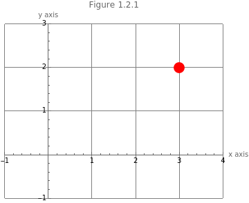
A point is usually written as an uppercase letter, for instance . If there are more than one point, we use subscripts such as , ,…,. The subscript , is a member of the natural or counting numbers. The ordered tuple follows directly after the point name, with the values written in parentheses. As an example, we have the point, , which is shown as a red dot in Figure 1.2.1. The Graphics function is used to plot the point .
P
P
1
P
2
P
n
n∈
P(3,2)
P(3,2)
In[]:=
Graphics[{PointSize[0.05],Red,Point[{3,2}]},AxesTrue,AxesLabel{"x axis","y axis"},PlotLabel"Figure 1.2.1",ImageSizeMedium,GridLines->Automatic,PlotRange->{{-1,4},{-1,3}}]
Out[]=
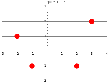
In Figure 1.2.2, we create four points, (3,2),(-2,1),(-1,-1), and (2,-1), one in each of the four quadrants of the Cartesian plane.
P
1
P
2
P
3
P
4
In[]:=
(*Creatingthepointsaslistobjectsassignedtoappropriatevariablenames*)={3,2};={-2,1};={-1,-1};={2,-1};
P
1
P
2
P
3
P
4
In[]:=
(*PlottingthefourpointsusingtheGraphicsfunction*)Graphics[{PointSize[0.05],Red,Point[{,,,}]},AxesTrue,PlotLabel"Figure 1.1.2",ImageSizeMedium,PlotRange->{{-3,4},{-2,3}},GridLines->Automatic]
P
1
P
2
P
3
P
4
Out[]=
Since every point above has two coordinates, we say that is an element of the set .
P
P
2
Points can exist in Cartesian space, , where we have three mutually orthogonal axes. We generate this space by adding a mutually perpendicular axis to the Cartesian plane, in accordance with the right-hand rule. Such a point is denoted as . There is no stopping, though, as points can exist in hyperspace, , where , and .
(x,y,z)∈
3
z
P(x,y,z)
n
,n>3
n∈
Enough about simple points. Let’s change our point of view.
1.3 Vectors
1.3 Vectors
Vectors have an algebraic and a geometric interpretation. In the geometric view, they are line segment between two points. This line segment has a start, termed the tail of the vector, and an end, termed the head of the vector. Vectors are also mathematical objects in their own right.
1.3.1 Vectors as geometric objects
1.3.1 Vectors as geometric objects
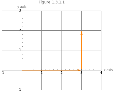
In the geometric view of a vector, we can imagine traveling from the origin, which we will denote as (0,0). We travel along the and then the axis by a distance as indicated by the values of the tuple of a point (the coordinates). Starting at the origin and traveling to the point above, we travel units along the axis and then up, units, along the axis.
P
o
x
y
P(3,2)
3
x
2
y
Since we are travelling, we can demonstrate our path with an arrow, with its tail at the starting position and its head and the end position. Our two paths are shown in Figure 1.3.1.1.
In[]:=
(*GeneratingthecomponentsforFigure1.3.1.1*)tailX={0,0};headX={3,0};tailY=headX;headY={3,2};
In[]:=
(*PlottingthetwovectorsasapathtothepointP(3,2)*)Graphics[{Orange,Thick,Arrow[{tailX,headX}],Arrow[{tailY,headY}]},AxesTrue,AxesLabel{"x axis","y axis"},PlotLabel"Figure 1.3.1.1",ImageSizeMedium,GridLines->Automatic,PlotRange->{{-1,4},{-1,3}}]
Out[]=
We can also simply travel in a straight line from the origin to the point as shown in Figure 1.3.1.2.
P(3,2)
In[]:=
Graphics[{{PointSize[0.03],Red,Point[{3,2}]},Orange,Thick,Arrow[{{0,0},{3,2}}]},AxesTrue,AxesLabel{"x axis","y axis"},PlotLabel"Figure 1.3.1.2",ImageSizeMedium,GridLines->Automatic,PlotRange->{{-1,4},{-1,3}}]
Out[]=
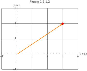
We have turned a point into a vector.
1.3.2 Vectors as mathematical objects
1.3.2 Vectors as mathematical objects
To print this list object as a column vector, we pass it as a parameter to the MatrixForm function.
1.4 Magnitude of a vector
1.4 Magnitude of a vector
With vectors as geometric objects, it is clear to understand that they must have length, termed a magnitude.
In the plane, such a magnitude can be calculated using the Pythagorean theorem. This is because we can complete a right-angled triangle from any vector, as shown in Figure 1.4.1.
Definition 1.4.1 The magnitude of a vector is defined as the square root of the sum of squares of each of the components of the vector, shown in (6).
We use the Norm function in the Wolfram Language to calculate the magnitude of a vector.
We verify this result using the Norm function.
1.5 Direction of a vector
1.5 Direction of a vector
We convert this to degrees.
Moving on to quadrant three in Figure 1.5.3, where we must get a negative angle.
We convert this to degrees.
Lastly, we have the fourth quadrant in Figure 1.5.4. where the angle must negative as well.
We convert this angle to radians as well.
1.6 Vector equality
1.6 Vector equality
Definition 1.6.1 Two or more vectors are equal vectors if and only of their components are the same or they have the same magnitude and direction.
So, the two vectors depicted in Figure 1.6.1, are exactly the same vector. In this case we speak about free vectors. A free vector is a vector that can be moved so that its tail coincides with the origin of the space in which it is in.
1.7 Unit vectors
1.7 Unit vectors
With the magnitude and direction of vectors defined, we can look at unit vectors.
This is accomplished by dividing each component of a vector by the magnitude of the vector, as shown in (8).
Problem 1.7.1
The norm or magnitude of the vector is calculated using the Norm function.
By dividing each component by the magnitude, we display the result as a column vector using the MatrixForm function.
In (9) we use scalar-vector multiplication, which we will learn about later.
Definition 1.7.2 The standard unit vectors are the unit vectors along the Cartesian axes.
1.8 Non-Cartesian coordinate systems
1.8 Non-Cartesian coordinate systems
While we commonly deal with Cartesian (or rectangular) coordinates, it may be more convenient to introduce non-rectangular coordinates in some cases. One or more parameters may remain constant or change in a predictable manner along these coordinates.
As an example we use the vector v from above, expressed again below for convenience.
When we pass the approximate values above as parameters, we return the original rectangular coordinates (within a margin of error).
As before we generate a function to do the coordinate transformation.
Conversion from spherical coordinates to Cartesian coordinates are shown in (17).
We also generate a function to return spherical coordinates to rectangular coordinates.
Passing the values from before as parameters, returns the approximate original rectangular coordinates.
The mutually perpendicular unit vectors are shown in (18).
The SphericalPlot3D function is used below to demonstrate the unit sphere in spherical coordinates in Figure 1.8.1.
1.9 Row vectors
1.9 Row vectors
The operation of the transpose, transforms a column into a row. Below, we use the Transpose function on v and print the result using the MatrixForm function.
1.10 Vector arithmetic
1.10 Vector arithmetic
As mathematical objects, we can perform arithmetic with vectors. These are simple to do and have an intuition from the geometric view of a vector. There are two operations defined on vectors. Vector addition and scalar-vector multiplication.
1.10.1 Vector addition
1.10.1 Vector addition
We have already seen vector addition in actions, where we add the corresponding components of two vectors to each other in Figure 3 and Figure 4. Note that vectors can only be added if they exist in the same space (with a similar number of components). We cannot add the two vectors in (19).
Definition 1.10.1.1 Vector addition is defined as the component-wise addition of the elements of two vectors in the same space, shown in (20).
The zero vector is a neutral element, or additive identity, with the property shown in (24).
Next, we consider scalar multiplication.
1.10.2 Scalar-vector multiplication
1.10.2 Scalar-vector multiplication
Definition 1.10.2.1 Scalar-vector multiplication is the component-wise multiplication of each component of the vector by the indicated scalar, shown in (25).
This means that we have the equality in (26), where scalar-vector multiplication is simply the scaling of the magnitude of a vector.
This reversal of direction is seen in Figure 1.10.2.2.
1.10.3 Vector subtraction
1.10.3 Vector subtraction
We can now do vector subtraction by adding this inverse. Since we are adding a vector and its additive inverse, the result is the zero vector.
We see the result in Figure 14 and verify it with code. The original two vectors are in green and their difference in orange. We also the the sum of the two vectors in the dotted blue vector. The dotted pink line is the free vector of the difference between the two vectors.
1.10.4 Vector dot product
1.10.4 Vector dot product
Problem 1.10.4.1 Calculate the dot product between the vectors in (19).
We see the solution in (20), using the definition in (18).
The Dot function performs the dot product.
The solution is calculate in (31).
We verify the result in the code cell below.
We note that the dot product of a vector with itself is the square of it magnitude, shown in (32).
1.10.5 The dot product as a function of the angle between vectors
1.10.5 The dot product as a function of the angle between vectors
The dot product can be redefined as a function of the angle between two vectors. This requires the law of cosines. Wolfram Alpha gives us information on this law.
In[]:=
Law of cosines
The solution is shown in (35).
We can verify the result using the ArcCos function.
For a numerical approximation, we use the N function.
Below, we combine the N and VectorAngle function for more succinct code.
1.10.6 Cauchy-Schwarz inequality
1.10.6 Cauchy-Schwarz inequality
Definition 1.10.6.1 The Cauchy-Schwarz inequality is defined in (36).
This states that the absolute value of the dot product of two vectors is less than or equal to the product of the magnitude of the two vectors.
We confirm the inequality for this example below.
1.10.7 Minkowski triangle inequality
1.10.7 Minkowski triangle inequality
This inequality is intuitively understood from the three sides of a triangle. If two sides are interpreted as two vectors, arranged tail-to-head, so as to indicate the sum of the two vectors, then the length of these two sides is equal to or longer than their addition.
Definition 1.10.7.1 The Minkowski inequality or the triangle inequality is defined in (37).
We do this comparison in code below and confirm the inequality for this example..
1.10.8 Orthogonal projections
1.10.8 Orthogonal projections
We can also derive the magnitude of this projection, shown in (27).
1.10.9 Vector cross product
1.10.9 Vector cross product
The result is another vector that is perpendicular (orthogonal) to the plane formed by the original two vectors.
The cross product is easily calculated from the determinant (which we will learn about in a later notebook) where we create a matrix (next notebook) with the first row being the standard unit vectors and the subsequent rows are the two vectors.
The reason for this is clear when we consider the angle between vectors. It should be clear, though, that parallel vector seen as position vectors are coincident and we cannot define a vector that is uniquely orthogonal to this.
Problem 1.10.9.1 Calculate the cross product between the vectors in (41).
The result in (42) is calculated using (40).
The result is confirmed using the Cross function and displaying the result in matrix form using the MatrixForm function.
We see the solution in Figure 1.10.9.1.
1.10.10 Scalar triple product
1.10.10 Scalar triple product
1.11 Spanning
1.11 Spanning
1.12 Complex vectors
1.12 Complex vectors
1.12.2 Multiplication of two complex numbers
1.12.2 Multiplication of two complex numbers
The multiplication of two complex numbers follows a similar paradigm as their real counterparts.
The solution is shown in (50).
We use the Wolfram Language to verify this solution.
1.12.3 The complex conjugate of a complex number and complex number division
1.12.3 The complex conjugate of a complex number and complex number division
The solution is shown in (52).
We use the Wolfram Language to verify this solution.
1.12.4 The norm of a complex number
1.12.4 The norm of a complex number
The norm is calculated in (54) using (53).
The Norm function is used to verify the norm of the complex number.
1.12.5 The principle argument of a complex number
1.12.5 The principle argument of a complex number
The result is expressed as a decimal approximation using the N function. The ArcTan function is used as demonstrated in (49).
1.12.6 The transpose of a complex vector
1.12.6 The transpose of a complex vector
Problem 1.12.6.1 Calculate the transpose of the complex vector in (57).
The solution is given in (58).
We verify this solution using the Wolfram Language.
1.12.7 Dot product of two complex vectors
1.12.7 Dot product of two complex vectors
The solution is shown in (61).
We use the Wolfram Language to verify this solution.