3 | Systems of equations
3 | Systems of equations
This chapter of Linear Algebra by Dr JH Klopper is licensed under an Attribution-NonCommercial-NoDerivatives 4.0 International Licence available at http://creativecommons.org/licenses/by-nc-nd/4.0/?ref=chooser-v1 .
3.1 Introduction
3.1 Introduction
In this chapter, we learn how to solve linear equations. These equations form a system such that they have a solution or solutions that solve all of the equations at once. By learning new notation and applying some school algebra (with a twist), we can solve these equations in no time.
In this section we start in 2-space. This is the familiar plane with two variables, and . Linear equations in 2-space gives us lines and linear equations in 3-space gives us planes.
x
y
3.2 Linear systems
3.2 Linear systems
Definition 3.2.1 A linear equation is an algebraic equation in variables in which each term is either a constant or the product of a constant, , and one of the variable, , that is . The variables in the equation are raised to the power of one, and there are no product terms involving multiple variables.
n
c
n
n
i
c
i
n
i
Definition 3.2.2 A system of linear equations or a linear system is a set of linear equations.
The two equations in (1) below were created so that a single value for and a single value for solve both equations. Together, they make a system of linear equations.
x
y
y=7-xy=-2+
x
2
(
1
)We can plot these functions, shown in Figure 3.2.1. Since both are linear equations, the two equations are two lines. We find a common solution to the system where they intersect.
In[]:=
Plot7-x,-2+,{x,2,10},PlotLabel"Figure 3.2.1 Visual solution to a linear system",PlotLegends"Expressions",GridLines{{5,6,7},{0,1,2}},ImageSize->Medium
x
2
Out[]=
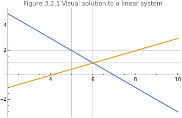
We see that they intersect at and , a perfect solution to our system of (two) linear equations.
x=6
y=1
We can rewrite this system of linear equations in matrix form. We start by rewriting our two equations using simple algebraic manipulations, (2).
x+y=7-x+2y=-4
(
2
)We can write the coefficients of the two left-hand sides as a matrix of coefficients and call it matrix , (3).
A
A=
1 | 1 |
-1 | 2 |
(
3
)We can write the unknowns as a column vector , (4).
x
x=
x |
y |
(
4
)The right-hand side solutions can also be written as a column vector , shown in (5).
b
b=
7 |
-4 |
(
5
)Now we can rewrite our problem in the notation of linear algebra, (6), using the properties and definitions of matrix-vector multiplication that we encountered in the last chapter.
Ax=b
=
1 | 1 |
-1 | 2 |
x |
y |
7 |
-4 |
(
6
)The aim is to find a solution for . We can do this if we can find an inverse for , namely . We will see that it has the property (if it exists) such that A=I, the identity matrix. A solution for , would therefor be as shown in (7).
x
A
-1
A
-1
A
x
-1
A
-1
A
-1
A
-1
A
(
7
)Above, we followed algebraic principles by applying a calculation on both sides of the equation (matrix multiplying by ). Because we have to be cognizant of commutativity, we do it in the same order on both sides (the goes first).
-1
A
-1
A
3.3 Introduction to the inverse of a matrix
3.3 Introduction to the inverse of a matrix
In this section, we solve a linear system by considering the inverse of a matrix. We learned of the existence of a matrix inverse in the previous chapter, when we noted that there is no such operation as matrix division. We have seen that the inverse matrix of a square matrix , is written as , such that it has the property shown in (8).
A
n×n
-1
A
n×n
A
n×n
-1
A
n×n
-1
A
n×n
A
n×n
I
n
(
8
)For , the inverse is easily calculated and is shown in (9).
n=2
A
2×2
a 11 | a 12 |
a 21 | a 22 |
-1
A
2×2
1
a
11
a
22
a
12
a
21
a 22 | - a 12 |
- a 21 | a 11 |
(
9
)The fraction in front of the altered matrix is known as the determinant. We will learn much more about it in the next chapter. From this fraction, though, it should be clear that there are matrices that will not have an inverse, i.e. when the elements of the matrix are such that the denominator is .
0
Below, we create matrix to investigate, (10). We follow the calculations established in (9) to calculate the inverse, .
A
-1
A
A=
=
=
=
1 | 1 |
-1 | 2 |
-1
A
1
1·2-1·(-1)
2 | -1 |
1 | 1 |
-1
A
1
3
2 | -1 |
1 | 1 |
-1
A
2 3 | - 1 3 |
1 3 | 1 3 |
(
10
)Now, we create this matrix in code.
In[]:=
matrixA={{1,1},{-1,2}};(*CreatingalistobjectassignedtothevariablematrixA*)MatrixForm[matrixA](*Printingthelistobejctasamatrix*)
Out[]//MatrixForm=
1 | 1 |
-1 | 2 |
The Inverse function calculates the inverse of a matrix.
In[]:=
MatrixForm[Inverse[matrixA]](*Printingthematrixformoftheinverseofthelistobject*)
Out[]//MatrixForm=
2 3 | - 1 3 |
1 3 | 1 3 |
For , the process is much more involved and we will deal with it later. For now, let’s reconsider the equation for our linear system. We are trying to solve for .
n>2
Ax=b
x
If we know the inverse of the matrix of coefficients, then we can solve a linear system (if an inverse exists). Let’s reconsider our very first linear system, reproduced in (11).
1x+1y=7-x+2y=-4
(
11
)The matrix of coefficients, the vector of unknowns, and the right-hand side vector is shown in (12). Don’t confuse the vector and it first component .
x
x
A=
,x=
,b=
1 | 1 |
-1 | 2 |
x |
y |
7 |
-4 |
(
12
)We have already used the Wolfram Language to solve for the inverse of and stored it as the list object inverseA. Below, we also create the vector as a list object assigned to the variable bVector and print it to the screen.
A
b
In[]:=
bVector={7,-4}(*Creatingalistobjecttoholdtheright-handsidevector*)
Out[]=
{7,-4}
Finally, we calculate b.
-1
A
In[]:=
MatrixForm[inverseA.bVector](*Pritingthesolutionofthevectorofunknowns*)
Out[]//MatrixForm=
6 |
1 |
We note the solution and . This does indeed solve our linear system as we saw in Figure 3.2.1, where the intersection of the two lines were at the point .
x=6
y=1
(6,1)
The other properties of the inverse matrix are listed in (13-14), assuming that they exist.
-1
(AB)
-1
B
-1
A
(
13
)-1
(kA)
-1
k
-1
A
(
14
)We can prove (13) by contradiction, where we first assume the there is no equality. This will give rise to a contradiction, which means that our assumption was false and that there is equality, (15). We make use of the properties of matrix-matrix multiplication, associativity, and matrix-inverse matrix multiplication.
-1
(AB)
-1
B
-1
A
-1
(AB)
-1
BB
-1
A
-1
(AB)
-1
A
-1
(AB)
-1
AA
-1
(AB)
(
15
)Since we have arrived at a contradiction, our initial assumption was false and =.
-1
(AB)
-1
B
-1
A
3.4 Linear systems with infinitely many solutions
3.4 Linear systems with infinitely many solutions
Let’s create a linear system with two unknowns and look at the outcome. We decide on the two values for the unknowns and add the coefficients to create the system, as shown in (16).
x=3,y=-54(3)+3(-5)=-32(3)+(-5)=-4x+3y=-3y=-x-12x+y=-y=-2x-y=-x-1
3
2
3
2
4
3
3
2
3
2
3
2
3
2
4
3
(
16
)We immediately see that we have the same equation and will have infinitely many solutions, shown in Figure 3.4.1.
In[]:=
Plot-x,-x,{x,-5,5},PlotLabel"Figure 3.4.1 Infinitely many solutions (lines are coincident)",PlotLegends"Expressions",ImageSize->Medium,GridLines->Automatic
4
3
4
3
Our matrix of coefficients shows us the problem as we use (9) to look at the determinant, (17).
Definition 3.4.1 A square matrix that is not invertible is a singular matrix.
3.5 Linear systems with no solutions
3.5 Linear systems with no solutions
It should be clear that two equations (in two unknowns) that are represented by parallel lines, but different intercepts, will have no solutions at all.
In Figure 3.5.1 we plot two such equations.
The matrix of coefficients will also not have an inverse and is a singular matrix as well.
3.6 Homogeneous linear systems
3.6 Homogeneous linear systems
Definition 3.6.1 A homogeneous linear system has the property shown in (18).
Let’s create a linear system, starting again by stating the solutions, (19).
Our linear system is shown in (20).
The only solution is the zero vector, a trivial solution. This is a property of homogeneous linear systems. If the matrix of coefficients is invertible then the homogeneous system only has the trivial solution.
Let’s have a look at an example in 3-space. We skip a few steps and set up a matrix of coefficients assigned to the computer variable coefficientMatrix using the Wolfram Language.
The inverse of this matrix is calculated below using the Inverse function and assigned to the variable inverseMatrix.
This matrix is invertible and for a homogeneous linear system, we will only have the trivial solution.
We will revisit the topics of infinitely many solutions and the trivial solution when we look at solving linear systems using augmented matrices.
3.7 Elementary row operations
3.7 Elementary row operations
In this section, we develop a systematic approach to solving linear systems. We will use a series of steps. There are only three steps and they are called elementary row operations. We can combine them in any order to solve our linear system problems.
These elementary row operations are nothing other than algebraic manipulation of the equations, rewritten in the notation of linear algebra.
We start with the concept of an augmented matrix. Here, we add the right-hand side to the matrix of coefficients in a single matrix. Our linear system is shown in (22).
The augmented matrix is shown in (23).
We start with the operation of interchanging the equations, (24).
Our augmented matrix will therefor be as in (25).
Now, we can do the third elementary row operation. Adding one row to another. Below, we do this by adding the first equation to the second (leaving the first equation intact), shown in (27).
These leading coefficients are called pivots. A concept that we will learn more about when we look at vector spaces.
The RowReduce function will do Gauss-Jordan elimination for us.
3.8 Elementary matrices
3.8 Elementary matrices
In another approach to understanding the solutions to linear systems through the use of matrices and elementary row operations, we consider elementary matrices in this section. An elementary matrix is the result of performing an elementary row operation on an identity matrix.
Note what happens if we multiply the original matrix of coefficients with this first elementary matrix.
3.9 Solving systems of linear equations using augmented matrices
3.9 Solving systems of linear equations using augmented matrices
We have seen how to use elementary row operations to solve linear systems. In this section, we look at the solutions when using them on augmented matrices representing various linear systems.
For some linear systems, either an infinite number of solutions or no solutions exists. The first occurs when the two lines are incident upon each other. In the example shown in (16), note that the second equation is simply a constant multiple of the other. Below is the same example as we saw in (16), recreated here in (36).
In (37), we look at Gauss-Jordan elimination of the augmented matrix of this linear system.
We can plot all these solutions using the ParametricPlot function, shown in Figure 3.9.1.
The linear system in (40), will have no solutions as the slope of the two lines are the same.
The augmented matrix in reduced row-echelon form is calculated below.
3.10 Disproportionate equations and unknowns
3.10 Disproportionate equations and unknowns
While it is simple enough to work with square matrices of coefficients, representing a linear system with the same number of equations and unknowns, we are not always in such a position.
Below, we create a linear system with three equations in two unknowns, (41).
This system has a unique solution as we can see in Figure 3.10.1.
The reduced row-echelon form shows the redundance of the third row.
In (42), we have three unknowns, but only two equations.
We see the plot of the two planes in Figure 3.10.2 and note the line of intersection, which means there are infinitely many solutions.
The reduced row-echelon form is shown below.
3.11 Calculating the inverse using elementary row operations
3.11 Calculating the inverse using elementary row operations
We can calculate the inverse of a matrix adding the identity matrix to a square matrix.
Below, we create a matrix, (47), and calculate its inverse.
In (48), we use elementary row operations to calculate the inverse. Note how the identity matrix is added to the original matrix. The original matrix turns into an identity matrix and the identity matrix turns into the inverse.
The inverse is now read from the original identity matrix.
3.12 LU decomposition
3.12 LU decomposition
Matrix decomposition is an important task in linear algebra. We decompose a matrix into other matrices, such that their composition (multiplication) gives us the original matrix. The first such decomposition that we will look at is LU decomposition. The LU stands for lower-upper decomposition, where we decompose matrices to triangular forms.
Definition 3.12.1 A triangular matrix has all 0 entries for elements above (lower triangular) or below (upper triangular) the main diagonal.
The matrix in (49) is upper triangular.
We can use the UpperTriangularMatrixQ function to check on this.
Note that these matrices need not be square. Below, we look at the same matrix as above, but add an extra row of all 0 elements (50).
The matrix in (51) is also upper triangular.
The transpose of an upper triangular matrix is lower triangular.
We can use the elementary matrices to decompose a matrix into upper triangular form. This is achieved by Gauss elimination. We revisit the matrix we used in the previous section on elementary matrices.
Our first three elementary matrices remain the same.
Depending on the elementary row operations used, a different set of elementary matrices will be created, leading to a different LU decomposition. Below, we use the LUDecomposition function to calculate an LU decomposition.
Notice that the multiplication of these matrices still gives us the same original matrix.