5 | Euclidean space
5 | Euclidean space
This chapter of Linear Algebra by Dr JH Klopper is licensed under an Attribution-NonCommercial-NoDerivatives 4.0 International Licence available at http://creativecommons.org/licenses/by-nc-nd/4.0/?ref=chooser-v1 .
5.1 Introduction
5.1 Introduction
We return to our study of vectors, with the goal of defining vector spaces in the next chapter. In this notebook, we restrict ourselves to Euclidean space and explore the uses of vectors ans vector arithmetic in Euclidean space.
5.2 Euclidean n-space
5.2 Euclidean -space
n
To start this notebook, let us review the definitions of vector arithmetic and the properties of vectors over the field of real numbers, .
5.2.1 Definitions of vector arithmetic
5.2.1 Definitions of vector arithmetic
Definition 5.2.1.1 Consider the definition of vectors, , in (1) that we will use in this chapter.
u,v∈
n
u=
,v=
u 1 |
u 2 |
⋮ |
u n |
v 1 |
v 2 |
⋮ |
v n |
(
1
)Definition 5.2.1.2 We define scalar-vector multiplication in (2) for a scalar .
c∈
cu=
cu 1 |
cu 2 |
⋮ |
cu n |
(
2
)Definition 5.2.1.3 If we have that , the additive inverse of follows, (3).
c=-1
u
(-1)u=
=-u
- u 1 |
- u 2 |
⋮ |
- u n |
(
3
)Definition 5.2.1.4 We now have a definition for vector addition, shown in (4), and vector subtraction, shown in (5).
u+v=
+
=
u 1 |
u 2 |
⋮ |
u n |
v 1 |
v 2 |
⋮ |
v n |
u 1 v 1 |
u 2 v 2 |
⋮ |
u n v n |
(
4
)u-v=u+(-v)=
-
=
+
=
u 1 |
u 2 |
⋮ |
u n |
v 1 |
v 2 |
⋮ |
v n |
u 1 |
u 2 |
⋮ |
u n |
- v 1 |
- v 2 |
⋮ |
- v n |
u 1 v 1 |
u 2 v 2 |
⋮ |
u n v n |
(
5
)Definition 5.2.1.5 We also the have additive identity vector, or the zero vector, , shown in (6).
o
o=
u+o=
+
=
=u
0 |
0 |
⋮ |
0 |
u 1 |
u 2 |
⋮ |
u n |
0 |
0 |
⋮ |
0 |
u 1 |
u 2 |
⋮ |
u n |
(
6
)5.2.2 Properties of vectors in n
5.2.2 Properties of vectors in
n
From the definitions above, we have the following summary of the properties of , , and , all elements of , and , , , and , all elements of , listed in (7).
u
v
w
n
1
c
c
1
c
2
u+v=v+u(u+v)+w=u+(v+w)u+0=uu+(-u)=0(u)=()uc(u+v)=cu+cv(+)u=u+u1u=u
c
1
c
2
c
1
c
2
c
1
c
2
c
1
c
2
(
7
)5.2.3 Dot product
5.2.3 Dot product
Definition 5.2.3.1 We defined the dot product of two vectors and in as in (8).
u
v
n
u·v=v=()∈
T
u
n
∑
i=1
u
i
v
i
(
8
)This gives is the properties of the dot product, listed in (9).
u·v=v·u(u+v)·w=u·w+v·w(cu)·v=c(u·v)u·u≥0u·u=0iffu=0
(
9
)The dot product can be redefined as a function of the angle between two vectors. Derivation of this requires the law of cosines. Wolfram|Alpha free-from input gives us information on this law.
In[]:=
Law of cosines
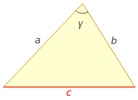
We make use of the norm of the difference between two vectors for our derivation, shown in (10). Here, , from the law of cosines above is equal to .
c
||u-v||
||u-v=++…+||u-v=-2++-2++…+-2+||u-v=(++…+)+(++…+)-2(++…+)||u-v=||u+||v-2||u-v=||u+||v-2(·)=+-2abcos(γ)||u-v=||u+||v-2[||u||||v||cos(γ)]u·v=||u||||v||cos(γ)γ=arccos
2
||
2
(-)
u
1
v
1
2
(-)
u
2
v
2
2
(-)
u
n
v
n
2
||
2
u
1
u
1
v
1
2
v
1
2
u
2
u
2
v
2
2
v
2
2
u
n
u
n
v
n
2
v
n
2
||
2
u
1
2
u
2
2
u
n
2
v
1
2
v
2
2
v
n
u
1
v
1
u
2
v
2
u
n
v
n
2
||
2
||
2
||
n
∑
k=1
u
k
v
k
2
||
2
||
2
||
u
v
2
c
2
a
2
b
2
||
2
||
2
||
u·v
||u||||v||
(
10
)We restrict ourselves to radians. So, if we want to calculate the angle between vectors and (, we can make use of (10). The
0≤γ≤π
T
(1,0)
T
1,1)
VectorAngle
function can do this calculation for us.In[]:=
VectorAngle[{1,0},{1,1}]
Out[]=
π
4
We create the two vectors as list objects assigned to the variables u and v. The VectorAngle function determines the argument and the N function expresses the result in approximate form.
5.2.4 Norm of a vector
5.2.4 Norm of a vector
Definition 5.2.4.1 The norm or the Euclidean length or the magnitude of a vector is defined in (11).
This brings us to a metric in Euclidean space.
5.2.5 Metric of distance in Euclidean space
5.2.5 Metric of distance in Euclidean space
The result is shown in ().
We confirm the results by creating to list object representing the two vectors and assigning them to the variables u and v.
5.2.6 Cauchy-Schwarz inequality
5.2.6 Cauchy-Schwarz inequality
The properties of the norm of a vector are shown in (16).
5.2.7 Minkowski triangle inequality
5.2.7 Minkowski triangle inequality
We can prove the inequality as shown below, (18).
Two other inequalities are shown in (19).
5.2.8 Pythagorean theorem
5.2.8 Pythagorean theorem
Definition 5.2.8 The Pythagorean theorem can be expressed using the norm of vectors, shown in (20).
5.3.1 Lines in 2-space
5.3.1 Lines in 2-space
We are all familiar with lines in the plane. It is usually expressed as the single variable equation shown in (23).
This allows us to express the line as a vector (25).
As example, we might want to express the line in (26) in parametric form. This is the line we plotted above.
We choose a simple parametrization (27).
5.3.2 Lines in 3-space
5.3.2 Lines in 3-space
This allows us to express the parametric equations for a line in 3-space, (29).
Problem 5.3.2.1 Find the parametric equations for a line in 3-space that passes through the two points in (32).
We can form a vector from these two points, (33).
The point of intersection is therefor as in (39).
5.3.3 Equations of planes
5.3.3 Equations of planes
The equation of the plane can also be found, given three points in the plane. We explore this through an example.
A point and a line in a plane can also be used to calculate the equation of the plane. We will also explore this using an example.
Problem 5.3.3.3 Find the equation of the plane given the point and the line in (48).
With the two points, we create another vector, this time, in the plane (49).
The cross product gives us a normal and we use the same steps as in the previous problem.
The solution is in (51).
One more way to find the equation of a plane is with two points in the plane and another plane perpendicular to it. This is also demonstrated using an example.
We can extract the normal to the perpendicular plane. Since it is orthogonal to this plane, it is parallel to the plane for which we seek an equation, (52).
We can create another vector in our plane from the two given points, (53).
Now we follow the same steps as before.
The solution is in (55).
5.3.4 Midpoints
5.3.4 Midpoints
We can write the components of this midpoint vector as a finite sequence, shown in (57).
Problem 5.3.4.1 Find the midpoint vector between the two vectors in (58).
The simple calculation follows in (59).
In Figure 5.3.4.1 we take a look at our two vectors and the midpoint vector.
5.3.5 Area of a parallelogram and triangle
5.3.5 Area of a parallelogram and triangle
Definition 5.3.5.1 The area of a parallelogram is the length of the base times the perpendicular height.
Constructing two sides of the parallelogram as vectors with a common initial base, we can use simple geometry.
Through simple trigonometry, we have the following for the area of a parallelogram, shown in (60).
The area of a triangle follows from this and is simply a half of the area of a parallelogram formed from the triangle.
The two vectors are created as list objects assigned to the variables u and v.
Below, we calculate the cross product between the two vectors using the Cross function and passing the two list objects as first two parameters. The Cross function is passed to the Norm function to calculate the magnitude or then the area of the parallelogram defined by the two vectors.
5.3.6 Scalar triple product
5.3.6 Scalar triple product
This can be used to calculate the volume of a parallelepiped in 3-space, which is the absolute value of the scalar triple product.
5.3.7 Lines of intersection between planes
5.3.7 Lines of intersection between planes
The line of intersection between two planes has a direction vector. This vector is orthogonal to the plane made by the two normals of the planes.
The direction vector of a line that is the intersection of the two planes, shown in (65), can be calculated from their normals. The concept of the lines of intersection between planes is demonstrated by example.
Problem 5.3.7.1 Find the line of intersection between the planes in (66).
We can plot the two planes, shown in Figure 5.3.7.1.
The two normals and their cross product is shown below using the Cross function.
We solve these two equations for two unknowns using the RowReduce function on the augmented matrix.
5.3.8 Distance between a point and a plane
5.3.8 Distance between a point and a plane
Consider the figure below.
Substituting, we get the equation for the distance between a point and a plane, shown in (71).
So, to solve for this problem, we need the equation of the plane and the point coordinate.
Problem 5.3.8.1 Consider the point and the plane in (72) and calculate the distance between the point and the plane.
The distance between them is solved in (73) by substituting into (71).
5.3.9 Distance between parallel planes
5.3.9 Distance between parallel planes
Problem 5.3.9.1 Calculate the distance between the two planes in (74).
5.3.10 Orthogonal projections
5.3.10 Orthogonal projections
We can also derive the norm of this projection, (77).
We create the vectors as list objects assigned to the variable w and a and use the calculations in (79) and (80).