Fourier Transform - continuous aperiodic signals
Fourier Transform - continuous aperiodic signals
Introduction to Fourier Transform
Introduction to Fourier Transform
We already know that the continuous periodic signal x (t) with period T can be represented by the Fourier complex series:
- is the complex amplitude for n=...-2,-1,0,1,2...
For aperiodic continuous signals we can assume that T = ∞. Then the factor (2 π) / T goes to zero and the sum becomes an integral:
Where is the complex continuous amplitude
- is the complex amplitude for n=...-2,-1,0,1,2...
For aperiodic continuous signals we can assume that T = ∞. Then the factor (2 π) / T goes to zero and the sum becomes an integral:
Where is the complex continuous amplitude
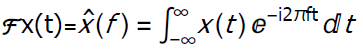
Fourier transfom is an integral transform from the time domain into the frequency domain. The transform is the result a of Fourier transformation ( the transformation is a mathematical operation on a function, resulting in th transform). We will take the notationis the Fourier transform of the function x (t). Transformation ℱacts on function x(t) and as a result we get a transform or function .is the inverse Fourier transform. Transformation ℱ^-1 acts on function as a result we get the reconstructed function x (t).
Fourier transformation is the basic tool for the harmonic analysis of functions, in which the complex exponential functions of the form are taken as elementary components . The transform determines the amplitudes (i.e. amount) of individual harmonics (frequencies) .
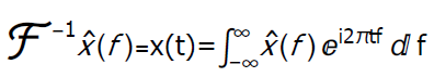
The step function is drawn below: to write a step function in Mathematica, we can use, the Piecewise [] or UnitStep [] function:
In[]:=
Plot[Piecewise[{{0, -∞ < t < -0.5}, {1, -0.5 <= t <= 0.5}, {0, 0.5 < t < ∞}}], {t, -1, 1}]
Out[]=
Out[]=
In[]:=
xt=Plot[UnitStep[(1/2-t)(1/2+t)],{t,-1,1},PlotLabel"signal"]
Out[]=
Out[]=
We use FourierTransform [] to determine Fourier transform in Mathematics
We use FourierTransform [] to determine Fourier transform in Mathematics
In[]:=
x1[ω_] := FourierTransform[Piecewise[{{0, -∞ < t < -0.5}, {1, -0.5 <= t <= 0.5}, {0, 0.5 < t < ∞}}], t, ω]
In[]:=
x2[ω_] := FourierTransform[UnitStep[(1/2 - t) (1/2 + t)], t, ω]
x1[ω]
x1[f]
x1[f]
Out[]=
0.797885Sin[0.5ω]
ω
Out[]=
0.797885Sin[0.5f]
f
In[]:=
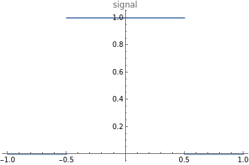
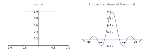
transx=Plot[x1[ω],{ω,-25,25},PlotLabel"Fourier transform of the signal"];
The step signal and its Fourier transform are presented below
GraphicsRow[{xt, transx}]
Out[]=
To calculate the inverse Fourier transform, use InverseFourierTransform []
InverseFourierTransform[x2[ω], ω, t]
FullSimplify[InverseFourierTransform[x2[ω], ω, t]]
FullSimplify[InverseFourierTransform[x2[ω], ω, t]]
Out[]=
2
π
1
2
π
2
1
2
1
2
π
2
1
2
Out[]=
1
2
1
2
1
2
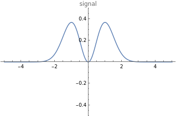
Another example
signal3 = Plot[t^2 Exp[-t^2], {t, -5, 5}, PlotRange -> {-0.5, 0.5}, PlotLabel -> "signal"]
Out[]=
transx3=Plot[Evaluate[FourierTransform[t^2Exp[-t^2],t,ω]],{ω,-10,10},PlotRange{-0.2,0.5},PlotLabel"Fourier transform of the signal"]
Out[]=
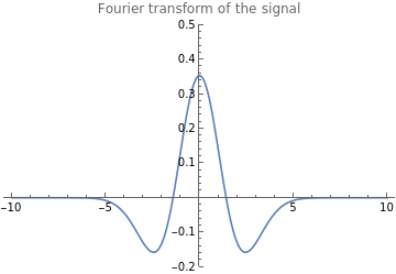
The signal and its Fourier transform are presented below
GraphicsRow[{signal3, transx3}]
Note that the above examples show real and even signals.
In addition, the Fourier transformation of the periodic function will be discrete, in the example below for the sine function we get the Dirac delta:
In addition, the Fourier transformation of the periodic function will be discrete, in the example below for the sine function we get the Dirac delta:
signal4 = Plot[Sin[t], {t, -5, 5}, PlotRange -> {-1.5, 1.5}, PlotLabel -> "signal"]
Note that the above examples show real and even signals
In addition, the Fourier transformation of the periodic function will be discrete, in the example below for the sine function we get the Dirac delta:
In addition, the Fourier transformation of the periodic function will be discrete, in the example below for the sine function we get the Dirac delta: