4.3 Non-Linear Regression Models
4.3 Non-Linear Regression Models
4.3.1 Polynomial Regression
4.3.1 Polynomial Regression
In[]:=
session=StartExternalSession["Python"]
Out[]=
ExternalSessionObject

Test
In[]:=
5+6
Out[]=
11
In[]:=
import numpy as np
X = np.sort(5 * np.random.rand(40, 1), axis=0)
y = np.sin(X).ravel()
y[::5] += 3 * (0.5 - np.random.rand(8))
X = np.sort(5 * np.random.rand(40, 1), axis=0)
y = np.sin(X).ravel()
y[::5] += 3 * (0.5 - np.random.rand(8))
In[]:=
np.savetxt('E:\\dX.txt',X,fmt='%.5e')
In[]:=
np.savetxt('E:\\yX.txt',y,fmt='%.5e')
In[]:=
Xt=Import["E:\\dX.txt","Table"];
In[]:=
yt=Import["E:\\yX.txt","Table"];
In[]:=
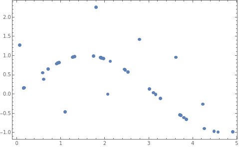
data=Transpose[{Flatten[Xt],Flatten[yt]}];
In[]:=
p0=ListPlot[data,Frame->True,PlotStyleTiny,Axes->None]
Out[]=
In[]:=
fitL=Fit[data,{1,x},x]
Out[]=
1.07846-0.327793x
In[]:=
fitP2=Fit[data,{1,x,x^2},x]
Out[]=
0.337505+0.628302x-0.202355
2
x
In[]:=
fitP3=Fit[data,{1,x,x^2,x^3},x]
Out[]=
0.194466+1.01029x-0.407103+0.0287582
2
x
3
x
In[]:=
fitP4=Fit[data,{1,x,x^2,x^3,x^4},x]
Out[]=
0.480557-0.313563x+0.852401-0.377213+0.0417352
2
x
3
x
4
x
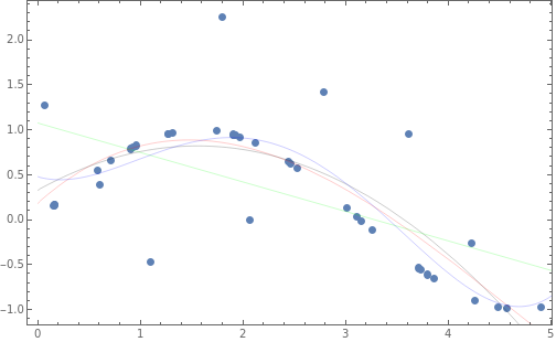
In[]:=
Show[{p0,Plot[fitP3,{x,0,40},PlotStyle{Thin,Red}],Plot[fitP2,{x,0,40},PlotStyle{Thin,Black}],Plot[fitL,{x,0,40},PlotStyle{Thin,Green}],Plot[fitP4,{x,0,40},PlotStyle{Thin,Blue}]}]//Quiet
Out[]=
In[]:=
from sklearn.preprocessing import PolynomialFeatures
from sklearn.linear_model import LinearRegression
from sklearn.linear_model import LinearRegression
In[]:=
regr = LinearRegression()
quadratic = PolynomialFeatures(degree=2)
X_quadratic = quadratic.fit_transform(X)
quadratic = PolynomialFeatures(degree=2)
X_quadratic = quadratic.fit_transform(X)
In[]:=
clf=LinearRegression().fit(X_quadratic,y)
In[]:=
clf.intercept_
Out[]=
0.337504
In[]:=
clf.coef_
Out[]=
NumericArray
In[]:=
Normal[%]
Out[]=
{0.,0.628303,-0.202355}
In[]:=
fitP2
Out[]=
0.337505+0.628302x-0.202355
2
x
In[]:=
clf.predict(quadratic.fit_transform([[20]]))
Out[]=
NumericArray
In[]:=
Normal[%]
Out[]=
{-68.0386}
Using Mathematica,
In[]:=
fitP2/.x20
Out[]=
-68.0385
In[]:=
regr = LinearRegression()
cubic = PolynomialFeatures(degree=3)
X_cubic = cubic.fit_transform(X)
cubic = PolynomialFeatures(degree=3)
X_cubic = cubic.fit_transform(X)
In[]:=
clf=LinearRegression().fit(X_cubic,y)
In[]:=
clf.intercept_
Out[]=
0.194466
In[]:=
clf.coef_
Out[]=
NumericArray
In[]:=
Normal[%]
Out[]=
{0.,1.01029,-0.407102,0.028758}
In[]:=
clf.predict(cubic.fit_transform([[20]]))
Out[]=
NumericArray
In[]:=
Normal[%]
Out[]=
{87.6232}
In[]:=
fitP3/.x20
Out[]=
87.6243
4.3.2 Polynomial Regression
4.3.2 Polynomial Regression
In[]:=
from sklearn.svm import SVR
import numpy as np
import numpy as np
In[]:=
svr_poly = SVR(kernel='poly', C=1e2, degree=3)
svr_rbf = SVR(kernel='rbf', C=1e3, gamma=0.3)
svr_rbf = SVR(kernel='rbf', C=1e3, gamma=0.3)
In[]:=
y_poly = svr_poly.fit(X, y).predict(X)
In[]:=
y_rbf= svr_rbf.fit(X, y).predict(X)
In[]:=
y_poly
In[]:=
y_rbf
4.3.3 Boundary of Saturn Rings
4.3.3 Boundary of Saturn Rings