1.1 Principal Component Analysis
1.1 Principal Component Analysis
1.1.1 Principal Component
1.1.1 Principal Component
In[]:=
X=N[{{1,2},{2.2,3},{4,10}}];X//MatrixForm
Out[]//MatrixForm=
1. | 2. |
2.2 | 3. |
4. | 10. |
In[]:=
std[data_]:=Module[{datatr=Transpose[data]},Transpose[N[Table[Standardize[datatr[[i]]],{i,1,Length[datatr]}]]]];
In[]:=
Xstd=std[X];Xstd//MatrixForm
Out[]//MatrixForm=
-0.927173 | -0.688247 |
-0.132453 | -0.458831 |
1.05963 | 1.14708 |
In[]:=
MatrixPlot[Xstd]//Binarize
Out[]=
In[]:=
n=3;
In[]:=
S=(Xstd//Transpose).Xstd/(n-1);MatrixForm[S]
Out[]//MatrixForm=
1. | 0.957186 |
0.957186 | 1. |
In[]:=
Covariance[Xstd]
Out[]=
{{1.,0.957186},{0.957186,1.}}
In[]:=
Eigenvalues[S]
Out[]=
{1.95719,0.042814}
In[]:=
Eigenvectors[S]
Out[]=
{{-0.707107,-0.707107},{0.707107,-0.707107}}
In[]:=
pc=Xstd.Eigenvectors[S];pc//MatrixForm
Out[]//MatrixForm=
0.168946 | 1.14227 |
-0.230784 | 0.418101 |
0.0618385 | -1.56038 |
In[]:=
MatrixPlot[pc]//Binarize
Out[]=

In[]:=
z=PrincipalComponents[Xstd];MatrixForm[z]
Out[]//MatrixForm=
1.14227 | 0.168946 |
0.418101 | -0.230784 |
-1.56038 | 0.0618385 |
In[]:=
Map[Reverse[#]&,z]//MatrixForm
Out[]//MatrixForm=
0.168946 | 1.14227 |
-0.230784 | 0.418101 |
0.0618385 | -1.56038 |
In[]:=
Correlation[z]//MatrixForm
Out[]//MatrixForm=
1. | 0. |
0. | 1. |
In[]:=
pc.Inverse[Eigenvectors[S]]Xstd
Out[]=
True
1.1.2 Singular Value Decomposition
1.1.2 Singular Value Decomposition
In[]:=
{u,s,v}=SingularValueDecomposition[Xstd];
In[]:=
u//MatrixForm
Out[]//MatrixForm=
0.57735 | 0.57735 | 0.57735 |
0.211325 | -0.788675 | 0.57735 |
-0.788675 | 0.211325 | 0.57735 |
In[]:=
s//MatrixForm
Out[]//MatrixForm=
1.97848 | 0. |
0. | 0.292623 |
0. | 0. |
In[]:=
u.s//MatrixForm
Out[]//MatrixForm=
1.14227 | 0.168946 |
0.418101 | -0.230784 |
-1.56038 | 0.0618385 |
1.1.3 Karhunen-Loeve Decomposition
1.1.3 Karhunen-Loeve Decomposition
In[]:=
KL=KarhunenLoeveDecomposition[Transpose[Xstd],StandardizedTrue][[1]]//Transpose;MatrixForm[KL]
Out[]//MatrixForm=
1.14227 | 0.168946 |
0.418101 | -0.230784 |
-1.56038 | 0.0618385 |
In[]:=
Join[z,First[z]]
Out[]=
{{1.14227,0.168946},{0.418101,-0.230784},{-1.56038,0.0618385},1.14227,0.168946}
In[]:=
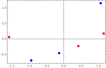
p0=Show[{ListPlot[Join[z,{First[z]}],PlotRangeAll,PlotStyle{PointSizeLarge,Red},AspectRatio0.65],ListPlot[Join[Xstd,{First[Xstd]}],PlotRangeAll,PlotStyle{PointSizeLarge,Blue},AspectRatio0.65]},PlotRangeAll,FrameTrue]
Out[]=
1.1.4 PCA and Total Least Square
1.1.4 PCA and Total Least Square
In[]:=
EigenvectorsX=Transpose[{Transpose[Eigenvectors[S]][[2]],{0,0}}]
Out[]=
{{-0.707107,0},{-0.707107,0}}
In[]:=
XstdX=z.PseudoInverse[EigenvectorsX]
Out[]=
{{-0.80771,-0.80771},{-0.295642,-0.295642},{1.10335,1.10335}}
In[]:=
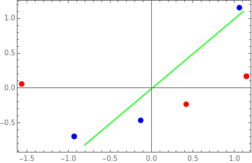
p1=Show[{p0,ListPlot[XstdX,JoinedTrue,PlotStyleGreen]}]
Out[]=
In[]:=
{x,y}=Transpose[Xstd];
In[]:=
obj=Apply[Plus,Table[+,{i,1,n}]];
2
Δx
i
2
(y[[i]]-α(x[[i]]-)-β)
Δx
i
1.1.5 Image Compression
1.1.5 Image Compression
1.1.6 Color Image Compression
1.1.6 Color Image Compression
1.1.7 Image Compression in Python
1.1.7 Image Compression in Python
Test
In[]:=
5+6
Source
Setup
In[]:=
from sklearn.decomposition import PCA
from sklearn.preprocessing import normalize
import scipy.io as sio
import matplotlib.image as image
import pandas as pd
import matplotlib.pyplot as plt
from sklearn.preprocessing import normalize
import scipy.io as sio
import matplotlib.image as image
import pandas as pd
import matplotlib.pyplot as plt
Load images
In[]:=
#Image is stored in MATLAB dataset
X = sio.loadmat('D:\\ex7faces.mat')
X = pd.DataFrame(X['X'])
#Normalize data by subtracting mean and scaling
X_norm = normalize(X)
X = sio.loadmat('D:\\ex7faces.mat')
X = pd.DataFrame(X['X'])
#Normalize data by subtracting mean and scaling
X_norm = normalize(X)
Run PCA
In[]:=
#Set pca to find principal components that explain 99%
#of the variation in the data
pca = PCA(.99)
#Run PCA on normalized image data
lower_dimension_data = pca.fit_transform(X_norm)
#Lower dimension data is 5000x353 instead of 5000x1024
lower_dimension_data.shape
#of the variation in the data
pca = PCA(.99)
#Run PCA on normalized image data
lower_dimension_data = pca.fit_transform(X_norm)
#Lower dimension data is 5000x353 instead of 5000x1024
lower_dimension_data.shape
Reconstruct images
In[]:=
#Project lower dimension data onto original features
approximation = pca.inverse_transform(lower_dimension_data)
#Approximation is 5000x1024
approximation.shape
#Reshape approximation and X_norm to 5000x32x32 to display images
approximation = approximation.reshape(-1,32,32)
X_norm = X_norm.reshape(-1,32,32)
approximation = pca.inverse_transform(lower_dimension_data)
#Approximation is 5000x1024
approximation.shape
#Reshape approximation and X_norm to 5000x32x32 to display images
approximation = approximation.reshape(-1,32,32)
X_norm = X_norm.reshape(-1,32,32)
Display Images
The following code displays the original images next to their 99% of variation counterparts. Because of how matplotlib displays images, the pictures may be rotated. If you really want to fix this, you can transpose each row of X_norm and approximation using a for loop.
The following code displays the original images next to their 99% of variation counterparts. Because of how matplotlib displays images, the pictures may be rotated. If you really want to fix this, you can transpose each row of X_norm and approximation using a for loop.
In[]:=
for i in range(0,X_norm.shape[0]):
X_norm[i,] = X_norm[i,].T
approximation[i,] = approximation[i,].T
fig4, axarr = plt.subplots(3,2,figsize=(8,8))
axarr[0,0].imshow(X_norm[0,],cmap='gray')
axarr[0,0].set_title('Original Image')
axarr[0,0].axis('off')
axarr[0,1].imshow(approximation[0,],cmap='gray')
axarr[0,1].set_title('99% Variation')
axarr[0,1].axis('off')
axarr[1,0].imshow(X_norm[1,],cmap='gray')
axarr[1,0].set_title('Original Image')
axarr[1,0].axis('off')
axarr[1,1].imshow(approximation[1,],cmap='gray')
axarr[1,1].set_title('99% Variation')
axarr[1,1].axis('off')
axarr[2,0].imshow(X_norm[2,],cmap='gray')
axarr[2,0].set_title('Original Image')
axarr[2,0].axis('off')
axarr[2,1].imshow(approximation[2,],cmap='gray')
axarr[2,1].set_title('99% variation')
axarr[2,1].axis('off')
plt.show()