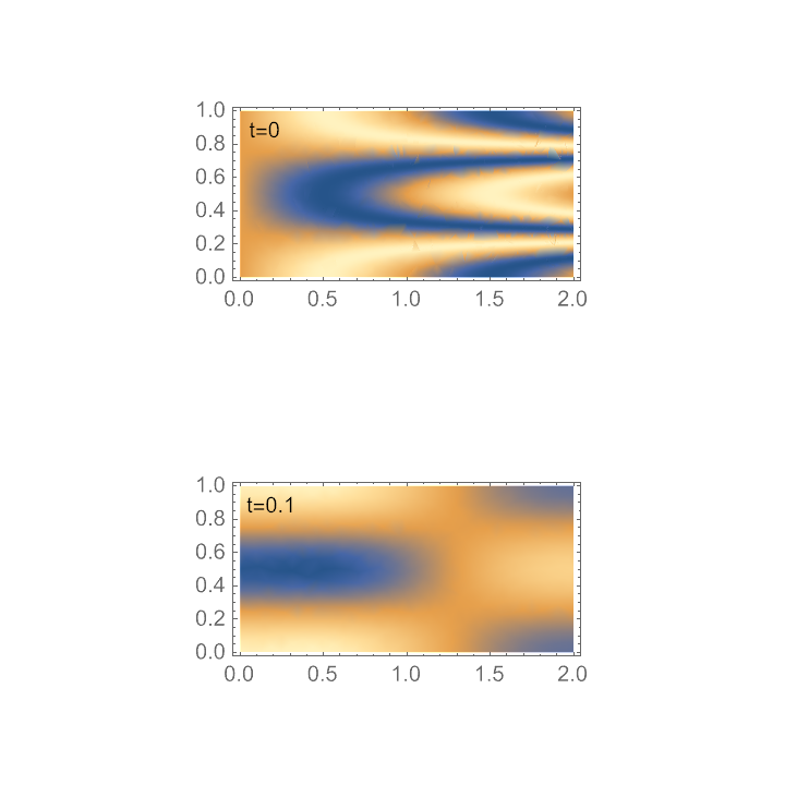
The heat equation describes how heat flows in a material. In this example we look at a 2D region over which we solve initial value problems to describe heat flow. We obtain both symbolic and numerical results for our solutions.

Define the heat equation: ∂_tu=∇²u in 2D:

In[1]:=

Out[1]=

Choose a region to solve the heat equation on:

In[2]:=

Out[2]=

Select an initial condition for the heat of the region as an arbitrary function:

In[3]:=

Out[3]=

Solve the heat equation on this region for the above initial conditions:

In[4]:=

Out[4]=

We see that the solution is just the same as the initial condition, but with a decaying exponential out front. This is because the initial condition could be separated into functions of each variable u[x,y,0]=f[x]g[y] with f[x]=Sin[2π x] and g[y]=Cos[π y]. What about an initial condition where this isn't true?

In[5]:=

Out[5]=

Let's add a periodic boundary condition since our initial condition is periodic in y:

In[6]:=

Solve the heat equation on Ω with this more complicated initial condition. This time use NDSolveValue to get a numerical result:

In[7]:=

Out[7]=

After just t=0.1, the higher frequency wiggles dissipated away and only the longer frequency wiggles survive:

In[8]:=

Out[8]=