◼
Nonlinear DDS have similiar input as Linear DDS but the computation takes longer to iterate. This produces larger time lags to compute p_n for large values of n.
◼
Nonlinear DDS often don't have a closed form analytic solution so we can't guarantee a shortcut when needing to compute large values of p_n
◼
We can often interpret the nonlinear dds by building it from the difference equation that tells the difference between the current output p_n and the previous output p_(n-1).
◼
Just like we had parameters "a" and "d" for the linear recursion equation, for a nonlinear recursion equation there are also parameters but we might assign different names.
◼
Part of the reason the recusion equation is non-linear is often because these parameters get multiplied by terms that depend on the independent variable which is the previous output p_(n-1).
◼
The Carrying Capacity Logistic Growth Model has two parameters R for Rate of Growth and C for Carrying Capacity
◼
Start by defining the initial condition and the recursion equation
In[]:=
p[0]=40;R=.8;Cap=500;p[n_]:=p[n-1]+R*(1-(p[n-1]/Cap))*p[n-1]
◼
Test an output
In[]:=
p[2]
Out[]=
117.277
◼
Output a table of values for n and p_n. NOTE: Be careful about iterating very far as the nonlinear computation takes more time. You may also choose to save the output with a variable name stored in memory that you can reference without having to recomput the table values every time.
In[]:=
mynonlindds=Table[{n,p[n]},{n,0,13}]
Out[]=
{{0,40},{1,69.44},{2,117.277},{3,189.092},{4,283.157},{5,381.398},{6,453.773},{7,487.336},{8,497.21},{9,499.43},{10,499.885},{11,499.977},{12,499.995},{13,499.999}}
Out[]=
{{0,40},{1,69.44},{2,117.277},{3,189.092},{4,283.157},{5,381.398},{6,453.773},{7,487.336},{8,497.21},{9,499.43},{10,499.885},{11,499.977},{12,499.995},{13,499.999}}
In[]:=
mynonlintab=TableForm[mynonlindds,TableHeadings{None,{"n iterations","p[n] output"}}]
Out[]//TableForm=
n iterations | p[n] output |
0 | 40 |
1 | 69.44 |
2 | 117.277 |
3 | 189.092 |
4 | 283.157 |
5 | 381.398 |
6 | 453.773 |
7 | 487.336 |
8 | 497.21 |
9 | 499.43 |
10 | 499.885 |
11 | 499.977 |
12 | 499.995 |
13 | 499.999 |
◼
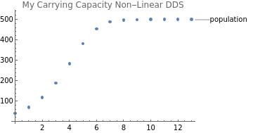
Here we plot the table output values, not the tableform command that displayed it in columns.
In[]:=
ListPlot[mynonlindds,PlotLabel"My Carrying Capacity Non-Linear DDS",PlotLabels"population"]
Out[]=
◼
We can build a manipulate interactive tool that allows you to adjust certain parameter values like the carrying capacity, growth rate, and initial conditions.
