◼
When we iterate a Discrete Dynamical System we define the recursion equation as a function and the initial condition
◼
A time series graph has our variable for time on the horizontal x axis and the output of our sequence p[n] on the vertical y axis.
◼
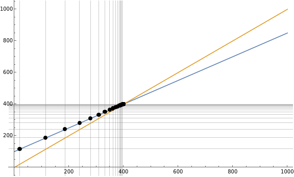
A fundamental graph depicts the previous output of the sequence that we defined as p[n-1] on the horizontal axis and the following output of the sequence on the vertical axis. A point (x,y) thus represents (p[n-1],p[n]) . This plot sometimes called a cobweb diagram because of the way we draw the DDS toward or away from the equilibrium value on it. We also draw two functions on our graph. One is the line where p[n-1]=p[n] or (x=y). The other is the line created by the recursion equation itself. Where the two lines intersect is the equilibrium value that we call p[*].
◼
Define a Discrete Dynamical system
In[]:=
p[0]=20;p[n_]:=.75*p[n-1]+100
◼
Show the outputs p[n] as n increass in a table
In[]:=
TableForm[Table[{n,p[n]},{n,0,35}]]
Out[]//TableForm=
0 | 20 |
1 | 115. |
2 | 186.25 |
3 | 239.688 |
4 | 279.766 |
5 | 309.824 |
6 | 332.368 |
7 | 349.276 |
8 | 361.957 |
9 | 371.468 |
10 | 378.601 |
11 | 383.951 |
12 | 387.963 |
13 | 390.972 |
14 | 393.229 |
15 | 394.922 |
16 | 396.191 |
17 | 397.144 |
18 | 397.858 |
19 | 398.393 |
20 | 398.795 |
21 | 399.096 |
22 | 399.322 |
23 | 399.492 |
24 | 399.619 |
25 | 399.714 |
26 | 399.786 |
27 | 399.839 |
28 | 399.879 |
29 | 399.91 |
30 | 399.932 |
31 | 399.949 |
32 | 399.962 |
33 | 399.971 |
34 | 399.979 |
35 | 399.984 |
◼
Here is a Times Series Graph of our Linear
In[]:=
ListPlot[Table[{n,p[n]},{n,0,35}],JoinedFalse]
Out[]=
◼
Now produce a table of outputs p[n] based on the input of the previous output p[n-1] . Note: Start at n=1 in the table so p[n-1] is initial condition p[0].
In[]:=
TableForm[Table[{p[n-1],p[n]},{n,1,35}]]
Out[]//TableForm=
20 | 115. |
115. | 186.25 |
186.25 | 239.688 |
239.688 | 279.766 |
279.766 | 309.824 |
309.824 | 332.368 |
332.368 | 349.276 |
349.276 | 361.957 |
361.957 | 371.468 |
371.468 | 378.601 |
378.601 | 383.951 |
383.951 | 387.963 |
387.963 | 390.972 |
390.972 | 393.229 |
393.229 | 394.922 |
394.922 | 396.191 |
396.191 | 397.144 |
397.144 | 397.858 |
397.858 | 398.393 |
398.393 | 398.795 |
398.795 | 399.096 |
399.096 | 399.322 |
399.322 | 399.492 |
399.492 | 399.619 |
399.619 | 399.714 |
399.714 | 399.786 |
399.786 | 399.839 |
399.839 | 399.879 |
399.879 | 399.91 |
399.91 | 399.932 |
399.932 | 399.949 |
399.949 | 399.962 |
399.962 | 399.971 |
399.971 | 399.979 |
399.979 | 399.984 |
◼
The plot of this table creates the values that go on the fundamental graph which displays how we advance the sequence based on the recursion equation.
In[]:=
ListPlot[Table[{p[n-1],p[n]},{n,1,35}]]
Out[]=
◼
To display a fundamental graph with the recursion equation line and the p[n-1]=p[n] or (x=y) we need to combine the previous scatter plot with a line plot.
In[]:=
Show[Plot[{.75x+100,x},{x,0,1000},PlotLegends"Expressions"],Graphics[{PointSize[Large],Red,Point[{100/(1-.75),100/(1-.75)}]}]]
Out[]=
◼
Combine the lines with the scatter plot points to see how we advance closer to the equilibrium value for this specific DDS.
In[]:=
Show[Plot[{.75x+100,x},{x,0,1000},PlotLegends"Expressions"],Graphics[{PointSize[Large],Red,Point[{100/(1-.75),100/(1-.75)}]}],ListPlot[Table[{p[n-1],p[n]},{n,1,35}],PlotStyleBlack]]
Out[]=
◼
We can add gridlines at the points to create a similiar effect depicted by a cobweb diagram. Start at the initial condition on the horizontal axis and go up to the recursion equation line and then over to the y=x line and then up to the recrusion equation line dot and keep repeating.
In[]:=
Show[Plot[{.75x+100,x},{x,0,1000},PlotLegends"Expressions",GridLines{Table[p[n-1],{n,1,16}],Table[p[n],{n,1,16}]}],Graphics[{PointSize[Large],Red,Point[{100/(1-.75),100/(1-.75)}]}],ListPlot[Table[{p[n-1],p[n]},{n,1,35}],PlotStyleBlack],ImageSizeLarge]
Out[]=
