Define Forward SDE
Define Forward SDE
Note that the SDE below is the simplest SDE we can think of in two dimensions just
x(t) = W1(t)
y(t) = W2(t)
the rest below is notation overhead with variable declaration
Note that the SDE below is the simplest SDE we can think of in two dimensions just
x(t) =(t)
y(t) =(t)
the rest below is notation overhead with variable declaration
x(t) =
W
1
y(t) =
W
2
the rest below is notation overhead with variable declaration
In[]:=
forwardsde=ItoProcess x[t][t], y[t][t] , {x[t],y[t]}, {{x,y},{,}}, t, WienerProcess[], WienerProcess[] ;
w
1
w
2
x
0
y
0
w
1
w
2
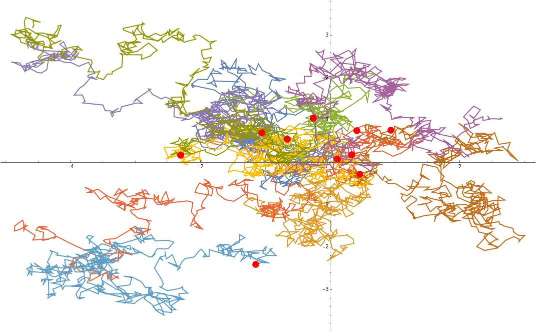
Now sample a few random points around (0,0) and see what happens...
Now sample a few random points around (0,0) and see what happens...
In[]:=
startpositions=RandomVariate[NormalDistribution[],{10,2}];
... put in SDE and caculate sample paths from time 0 up to 5
... put in SDE and caculate sample paths from time 0 up to 5
In[]:=
samplePathsWithTime=Table[RandomFunction[(forwardsde/.{,}->startpositions[[i]]),{0.,5.,0.01}],{i,Length[startpositions]}]//TemporalData
x
0
y
0
Out[]=
TemporalData
In[]:=
samplePathsPointsOnly=samplePathsWithTime["ValueList"];
In[]:=
Show[{ListLinePlot[samplePathsPointsOnly],ListPlot[startpositions,PlotStyle->Red]}]
Out[]=
Define a “complicated” probability distribution in two dimensions
Define a “complicated” probability distribution in two dimensions
In[]:=
mixturedist=MixtureDistribution,,{MultinormalDistribution[{-1,-1},{{1,0},{0,1}}],MultinormalDistribution[{2,5},{{1,0},{0,1}}]};
1
2
1
2
In[]:=
pdfxy[x_,y_]:=PDF[mixturedist,{x,y}]
In[]:=
pdfxy[x,y]
Out[]=
1
2
2
(-2+x)
2
(-5+y)
4π
1
2
2
(1+x)
2
(1+y)
4π
In[]:=
mynicePlot=Plot3D[pdfxy[x,y],{x,-10,10},{y,-10,10},PlotRange->All,PlotPoints->25,PlotTheme->"ZMesh"]
Out[]=

Now we go forward with the distribution
Now we go forward with the distribution
First we sample from our distribution, in real life the sample is given to us simply by the data, e.g. the CIFAR-10 pictures and we wouldn’t know the underlying distribution too well
First we sample from our distribution, in real life the sample is given to us simply by the data, e.g. the CIFAR-10 pictures and we wouldn’t know the underlying distribution too well
In[]:=
sampleFromMixture=RandomVariate[mixturedist,1000];
In[]:=
sampleFromMixturePlot=ListPointPlot3D[Append[#,0.1]&/@sampleFromMixture];
In[]:=
Show[mynicePlot,sampleFromMixturePlot]
Out[]=

check that the sample points correspond to our distribution by reconstructing the distribution from the points
check that the sample points correspond to our distribution by reconstructing the distribution from the points
In[]:=
kernelFromPoints=SmoothKernelDistribution[sampleFromMixture];
In[]:=
Plot3D[PDF[kernelFromPoints,{x,y}],{x,-10,10},{y,-10,10},PlotRange->All]
Out[]=

note that the correspondence here is quite good despite having only 1000 sample points
note that the correspondence here is quite good despite having only 1000 sample points
Now put initial points from our distribution in forward SDE and see what happens. Intuitively the points are shaken up and should lose all their correlations and gather in a simple standard normal around the origin (0,0) with some width (variance).
Now put initial points from our distribution in forward SDE and see what happens. Intuitively the points are shaken up and should lose all their correlations and gather in a simple standard normal around the origin (0,0) with some width (variance).
Plot endpoints of all paths, i.e. each particle has arrived somewhere in the plane
Plot endpoints of all paths, i.e. each particle has arrived somewhere in the plane
check if we have arrived at our simple normal distribution around origin by reconstruction distribution from end positions
check if we have arrived at our simple normal distribution around origin by reconstruction distribution from end positions
... not quite, but we have moved the distribution quite a bit when comparing with original
... not quite, but we have moved the distribution quite a bit when comparing with original
have to shake the points a little bit more, let’s go for 25 instead of 5
have to shake the points a little bit more, let’s go for 25 instead of 5
again check for distribution as before
again check for distribution as before
looks like a nice standard gaussian around origin
looks like a nice standard gaussian around origin
Some computations to get at the gradient field
Some computations to get at the gradient field
In real life we track the distributions with time in the forward process and learn the gradient field through a neural network. This is called score matching, because grad log of distribution is called “the score function”. Afterwards we have a black box function where we input position and time and it outputs the gradient.
Here we simply compute the gradient field analytically.
Here we simply compute the gradient field analytically.
We can intuitively see what it does: When used in the backward SDE it acts like a force field, forcing the particles despite the random forces in certain directions. So we still don’t know where each particle ends up, but the whole ensemble is forced to go in certain directions
We can intuitively see what it does: When used in the backward SDE it acts like a force field, forcing the particles despite the random forces in certain directions. So we still don’t know where each particle ends up, but the whole ensemble is forced to go in certain directions
Lets formulate backward SDE
Lets formulate backward SDE
we need the gradient of the log probability with time running backwards
we need the gradient of the log probability with time running backwards
we fit a standard gaussian with some width around our endpoints in order to sample from that distribution. Please note that we don’t use our endpoints to go backwards but sample totally new points from this easy distribution.
we fit a standard gaussian with some width around our endpoints in order to sample from that distribution. Please note that we don’t use our endpoints to go backwards but sample totally new points from this easy distribution.
Backward SDE
Backward SDE
New sample points now from our simple Gaussian we arrived at
New sample points now from our simple Gaussian we arrived at
Now go backward with these points
Now go backward with these points
Get the estimated distribution we arrived at, should match approximately the distribution we came from
Get the estimated distribution we arrived at, should match approximately the distribution we came from
Compare to original
Compare to original
Looks nice even with only 100 points
Looks nice even with only 100 points