◼
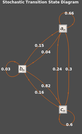
Defined our Matrix A of the transitions between states.
In[]:=
A=
.66 | .15 | .24 |
.04 | .03 | .16 |
.30 | .82 | .60 |
Out[]=
{{0.66,0.15,0.24},{0.04,0.03,0.16},{0.3,0.82,0.6}}
◼
This generates the diagram. You can change PlotTheme to other color combinations.
In[]:=
VertexReplace[DirectedGraph[AdjacencyGraph[Partition[ConstantArray[1,9],3]],VertexLabelsPlaced["Name",Center],EdgeLabelsTable[{"\!\(\*SubscriptBox[\(a\), \(n\)]\)""\!\(\*SubscriptBox[\(a\), \(n\)]\)","\!\(\*SubscriptBox[\(a\), \(n\)]\)""\!\(\*SubscriptBox[\(b\), \(n\)]\)","\!\(\*SubscriptBox[\(a\), \(n\)]\)""\!\(\*SubscriptBox[\(c\), \(n\)]\)","\!\(\*SubscriptBox[\(b\), \(n\)]\)""\!\(\*SubscriptBox[\(a\), \(n\)]\)","\!\(\*SubscriptBox[\(b\), \(n\)]\)""\!\(\*SubscriptBox[\(b\), \(n\)]\)","\!\(\*SubscriptBox[\(b\), \(n\)]\)""\!\(\*SubscriptBox[\(c\), \(n\)]\)","\!\(\*SubscriptBox[\(c\), \(n\)]\)""\!\(\*SubscriptBox[\(a\), \(n\)]\)","\!\(\*SubscriptBox[\(c\), \(n\)]\)""\!\(\*SubscriptBox[\(b\), \(n\)]\)","\!\(\*SubscriptBox[\(c\), \(n\)]\)""\!\(\*SubscriptBox[\(c\), \(n\)]\)"}[[i]]Style[Flatten[Transpose[A]][[i]],Bold,12],{i,1,9}],VertexShapeFunction"Square",VertexSizeMedium,VertexStyleLightBrown,VertexLabelStyle->Directive[Black,Italic,16],PlotTheme"Marketing",PlotLabelStyle["Stochastic Transition State Diagram",White,Bold]],{1"",2"",3""},GraphLayout"LayeredDigraphEmbedding"]
a
n
b
n
c
n
Out[]=
◼
Checked it was Stochastic because all columns equal one so nothing is coming from outside of our system and going into or out of the variable nodes in our system.
In[]:=
Total[A]
Out[]=
{1.,1.,1.}
◼
Define the systems of recursion equations to compute values of p_n based on our initial condition.
In[]:=
d={0,0,0};p[0]={620,0,0};p[n_]:=A.p[n-1];
In[]:=
p[1]
Out[]=
{409.2,24.8,186.}
In[]:=
p[7]
Out[]=
{248.163,61.3121,310.525}
◼
The inverse of I-A doesn’t exist because the A matrix is stochastic so we build the augmented matrix with the d vector as the last column and RowReduce to discover if infinite or no equilibrium vectors exist.
In[]:=
IdentityMatrix[3]-A//MatrixForm
Out[]//MatrixForm=
0.34 | -0.15 | -0.24 |
-0.04 | 0.97 | -0.16 |
-0.3 | -0.82 | 0.4 |
In[]:=
MatrixFormRowReduce
0.33999999999999997 | -0.15 | -0.24 | 0 |
-0.04 | 0.97 | -0.16 | 0 |
-0.3 | -0.82 | 0.4 | 0 |
Out[]//MatrixForm=
1 | 0. | -0.793082 | 0. |
0 | 1 | -0.197653 | 0. |
0 | 0 | 0 | 0 |
◼
Replace the Last Row with our equation based on the sum of our initial condition values. The sum of adding 100% of every variable adds up to the total number of items in our system because no new items enter or exit. This replaced the last row of all zeros as additional information about the particular equilibrium vector pstar that occurs based on our initial condition p[0].
In[]:=
RowReduce
1 | 0. | -0.7930821494749846 | 0. |
0 | 1 | -0.19765287214329832 | 0. |
1 | 1 | 1 | 620 |
Out[]=
{{1,0.,0.,247.},{0,1,0.,61.5576},{0,0,1,311.443}}
In[]:=
MatrixForm[%]
Out[]//MatrixForm=
1 | 0. | 0. | 247. |
0 | 1 | 0. | 61.5576 |
0 | 0 | 1 | 311.443 |
◼
You can can the pstar is an equilibrium vector by multiplying it by the matrix of coefficients A and getting the same result output p[n] that you input for p[n-1].
In[]:=
%53[[All,4]]
Out[]=
{247.,61.5576,311.443}
In[]:=
A.%53[[All,4]]
Out[]=
{247.,61.5576,311.443}
