◼
Practice solving systems of equations and matrix operations on a matrix A, a vector of unknown variables x and a solution vector b.
◼
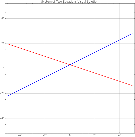
First begin with a system of 2 equations with 2 unkown variables x and y. An example would be 1 x + 3 y = 9 and -3 x + 6 y == 18. We can graph these equations visually
In[]:=
ContourPlot[{1x+3y==9,-3x+6y==18},{x,-50,50},{y,-50,50},AxesTrue,GridLinesAutomatic,PlotLabel"System of Two Equations Visual Solution",PlotLegendsAutomatic,ContourStyle{Red,Blue},ImageSizeLarge]
Out[]=
◼
The solution values for x and y that satisfy both equations are the value on the plot where the two lines meet.
◼
We could also define this system in a matrix vector form.
◼
Define Matrix A of coefficients for both equations .
In[]:=
A={{1,3},{-3,6}}
Out[]=
{{1,3},{-3,6}}
◼
Calculate several different operations on Matrix A.
In[]:=
MatrixForm[A]Length[A]IdentityMatrix[Length[A]]//MatrixFormTranspose[A]//MatrixFormDet[A]Tr[A]Inverse[A]//MatrixForm
Out[]//MatrixForm=
1 | 3 |
-3 | 6 |
Out[]=
2
Out[]//MatrixForm=
1 | 0 |
0 | 1 |
Out[]//MatrixForm=
1 | -3 |
3 | 6 |
Out[]=
15
Out[]=
7
Out[]//MatrixForm=
2 5 | - 1 5 |
1 5 | 1 15 |
◼
We could solve the system using the Solve command and inputting both equations
In[]:=
Solve[{1x+3y==9,-3x+6y==18},{x,y},Reals]
Out[]=
{{x0,y3}}
◼
We could also solve a system of equations for vector of unknowns x based on matrix vector product of Ax=b and solving for the unknown vector x.
◼
define solution vector b and unknown vector x
In[]:=
b={9,18}vecx={x,y}
Out[]=
{9,18}
Out[]=
{x,y}
◼
Solve the system using Solve command on the Ax=b equation to solve for vector of unknowns x. Here I called that vector vecx.
In[]:=
Solve[A.vecx==b,vecx]
Out[]=
{{x0,y3}}
◼
Confirm A Inverse exists by checking the determinant is not zero.
In[]:=
Det[A]
Out[]=
15
In[]:=
Inverse[A]
Out[]=
,-,,
2
5
1
5
1
5
1
15
◼
Since A inverse existed when checked above we take A Inverse matrix multiplied by solution vector b. the result will be the same
In[]:=
Inverse[A].b
Out[]=
{0,3}
◼
Finally we could solve by inputting the system of equations as an augmented matrix and doing elementary row operations using RowReduce. The last element of each row vector is part of the solution vector that corresponds to that equation. We hope to reduce the matrix on the left side to the identity matrix and the last column on the right to the values of the vector of unknowns that solves the system.
In[]:=
RowReduce[{{1,3,9},{-3,6,18}}]//MatrixForm
Out[]//MatrixForm=
1 | 0 | 0 |
0 | 1 | 3 |
◼
By several different techniques we have shown that the solution is when x=0 and y=3.
