Replacement rules for growing a planar network II
Replacement rules for growing a planar network II
2 May 2000
Matthew P. Szudzik
Initialization
Initialization
<<GraphLayout`GraphLayout`
Introduction
Introduction
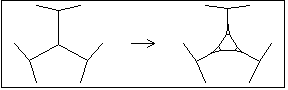
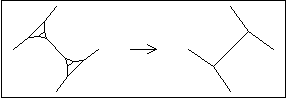
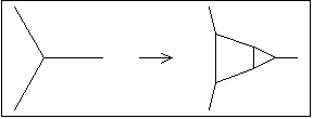
The network replacement rules and cause two-dimensional networks to "grow"—flattening two-dimensional hyperbolic or spherical networks. These replacement rules are derrived from a procedure that Andrew de Laix developed for flattening planar networks. His procedure involves finding the dual of a certain dissection of the faces in a planar network. The replacement rules implement the procedure as follows. transforms every node that lies between three faces, each of which has five or more sides, into a hexagon surrounded on three sides by connective structures. These connective structures are composed of squares and triangles whose presence temporarily prevents from being applied again. then removes the connective structures between hexagons, joining them together, and leaving a new network to which can once more be applied. The result of applying and then to a planar network (composed of faces with five or more sides) is that hexagons are inserted between all of the faces, increasing the size of the network and decreasing its curvature.
NodeToHexRule
HexJoinRule
NodeToHexRule
NodeToHexRule
HexJoinRule
NodeToHexRule
NodeToHexRule
HexJoinRule
NodeToHexRule
HexJoinRule
PNRuleGraphic
NodeToHexRule
NodeToHexRule={1{16,17,18},16{1,19,20},17{1,21,22},18{1,23,24}}{1{2,6,7},2{1,8,3},3{2,9,4},4{3,10,5},5{4,11,6},6{1,5,12},7{1,13,8},8{2,7,13},9{3,14,10},10{4,9,14},11{5,15,12},12{6,11,15},13{7,16,8},14{9,17,10},15{11,18,12},16{13,19,20},17{14,21,22},18{15,23,24}};
Show[Surround[PNRuleGraphic[NodeToHexRule]]];
HexJoinRule={1{2,3,4},2{1,5,6},3{1,7,4},4{1,3,8},5{2,9,6},6{2,5,10},7{3,11,8},8{4,7,12},9{5,13,10},10{6,9,14}}{1{2,14,11},2{1,12,13}};
Show[Surround[PNRuleGraphic[HexJoinRule]]];
These rules are designed so that causality is uniquely defined in the network, regardless of how the replacement rules are applied. That is, the causal network is independent of the order of evaluation. To demonstrate the results of applying these replacement rules, it is useful to apply the rules in two separate stages. If both rules were applied simultaneously, depending on the details of algorithm that is used to apply the rules, "time" may advance at different speeds in different regions of the network. Applying the rules in two separate stages guarantees that time advances at the same rate at all locations in the network.
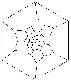
For example, consider applying the rules to a dodecahedron—the prototypical spherical network.
Show[PNGraphics[Spring[PNDodec]]];
A dodecahedron has 20 nodes.
Length[PNDodec]
20
The first stage applies until the network no longer changes.
NodeToHexRule
DodecStage1=Drop[FixedPointList[PNEvolveStep[{NodeToHexRule},#]&,PNDodec],-1];
Show[PNGraphics[Spring[DodecStage1[[-1]]]]];
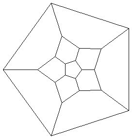
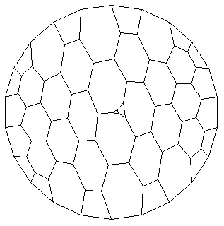
The second stage applies until the network no longer changes.
HexJoinRule
DodecStage2=Drop[FixedPointList[PNEvolveStep[{HexJoinRule},#]&,DodecStage1[[-1]]],-1];
Show[PNGraphics[Spring[DodecStage2[[-1]]]]];
The result is a larger (and flatter) network with 60 nodes.
Length[DodecStage2[[-1]]]
60
Evolution of Flat Space
Evolution of Flat Space
The function evolves the network for one time step.
PlanarGrowStep[net]
net
PlanarGrowStep[net_]:=FixedPoint[PNEvolveStep[{HexJoinRule},#]&,FixedPoint[PNEvolveStep[{NodeToHexRule},#]&,net]]
Consider an empty flat space evolved for three steps.
EmptySpaceInit=PNHexGrid[10,6];
EmptySpaceEvolve=NestList[PlanarGrowStep,EmptySpaceInit,3];
Localized Structures
Localized Structures
Because can only be applied to nodes on faces with five or more sides, structures composed of triangles and squares are localized structures that remain unaffected by the rule. It is therefore natural to interpret faces with five or more sides as "space" and faces with three or four sides as "matter". One immediate consequence of this identification is that the presence of matter increases the curvature of space—a property of the physical universe predicted by general relativity.
NodeToHexRule
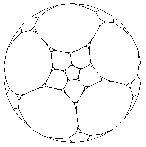
The introduction of creates a growing "wave-front" of particles.
Particle1
InsertParticle1={1{6,7,8}}{1{2,3,8},2{1,4,3},3{1,2,5},4{2,6,5},5{3,4,7}};
Show[Surround[PNRuleGraphic[InsertParticle1]]];
Particle1Init=PNEvolveStep[{InsertParticle1},PNHexGrid[10,10],{First,70,3}];
Show[PNGraphics[Spring[Particle1Init]]];
particle1=NestList[PlanarGrowStep,Particle1Init,3];
Show[PNGraphics[#]]&/@particle1;
The "swiss-cheese" connections near the outside is a temporal gradient—it signifies that the nodes in the interior are three time-steps ahead of the nodes around the edge.