Grubbs’ criterion

Created 10 March 2016 by Ronnie Mainieri.
Last updated 11 March 2016

Functions

Convert a list of numbers to units of standard deviation away from their mean.

studentize[data_List]:=Module[{mean,std},mean=Mean[data];std=StandardDeviation[data];(data-mean)/std]

Generate data that is distributed according to a Normal distribution with mean xbar and standard deviation sigma. If those values are not provided, it assumes 5 and 1.2.

generateData[n_Integer,xbar_,sigma_]:=Module[{m,data},data=RandomVariate[NormalDistribution[xbar,sigma],n];m=Mean[data];SortBy[data,Abs[#-m]&]];generateData[n_Integer]:=generateData[n,5,1.2]

Compute the critical value for establishing outliers for dataset that is supposed to be Normal distributed using Grubbs criterion when there are n data points and the two sided probability has to be no more than alpha.

criticalG[n_,alpha_]:=Module{r1,x,xc,tc,guess=2},xc=alpha(2n);r1=FindRoot[CDF[StudentTDistribution[n-2],x]1-xc,{x,guess}];(*Print[{x,1-CDF[StudentTDistribution[n-2],x]}/.r1];*)tc=x/.r1;

n-1

+n-2



Usage

To generate a sample of 7 random values sample from a Normal distribution with mean 5 and standard deviation of 1.2, one calls the function

data=generateData[7]

{4.25459,5.11813,4.18672,5.31024,5.38823,6.12194,2.37923}

The means and standard deviations of the sample need not agree with those of the population:

Mean[data]

4.67987

StandardDeviation[data]

1.21709

The function studentize takes a list of numbers and changes them to be in units of standard deviations from their mean

studentize[data]

{-0.34942,0.360088,-0.405189,0.517939,0.582012,1.18486,-1.89029}

Why remove outliers

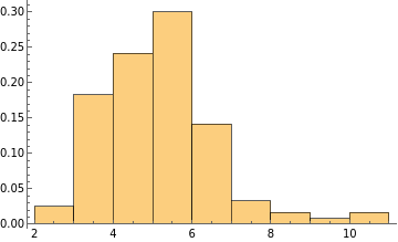
We start out by creating some simulation data of number picked from a Normal distribution with mean 5 and standard deviation of 1.2. We also “contaminate” it with numbers chosen from a Pareto distribution that has a long tail. These will play the role of outliers.

r1=RandomVariate[ParetoDistribution[4,1.5],20];r2=RandomVariate[NormalDistribution[5,1.2],100];h1=Join[r1,r2];

If we put a blue line for every data point we have, some points seem out of place.

The mean and the standard deviation of the sample are not those of the Normal distribution used in the simulation. The data does not resemble a Normal

The mean and standard deviations are far from the values of the Normal used in the simulation.

{m,sd}={Mean[h1],StandardDeviation[h1]}

{5.57831,2.52632}

The numbers coming from the Pareto distribution are highlighted in orange

Simulation

Suppose we have sample of 15 numbers and we want to identify the outliers. We will say that very small values or very large values are outliers if their studentized value is, in absolute value, bigger than gc. Using Grubbs’ criterion, that critical value is

gc=criticalG[15,0.05]

2.54831

We now run 100,000 simulations of picking 15 numbers and checking to see if any the set has any outliers

Table[If[(Abs@studentize@generateData[15])〚-1〛>gc,1,0],{100000}]//Total

5002

or about 5002/100000 = 5%. In other words, in a frequentist interpretation, using the Grubbs criterion in 5% of the cases we would have incorrectly classified the extreme point as an outlier.

Having more than one outlier is very rare in this case

d2=Table[Length@Select[studentize@generateData[15],(Abs[#]>gc)&],{100000}];

Tally[d2]

{{0,94998},{1,5002}}

Iterated Grubbs

Grubbs’s test only applies to question of whether the most extreme of points is an outlier. One may be tempted to use the test again with the one outlier removed, as is done with the function grubbsTrim. This function applies the Grubbs test until no further data points are removed.

grubbsTrim[h1_,g0_]:=Module[{oldLength,hn,guard,gc},oldLength=∞;guard=Length[h1];hn=h1;While[oldLength-Length[hn]≠0∧guard>0,--guard;oldLength=Length[hn];{m,sd}={Mean[hn],StandardDeviation[hn]};gc=g0sd+m;hn=Select[h1,(#<gc)&];];hn]

Applying the trimming procedure to the Normal data with the mixed in Pareto outliers, we end up removing a few points. For 120 points at 5% the studentized cutoff is

Comparing the resulting points with the ground truth, a few Pareto outliers still remain

but the estimates for the mean and standard deviation have smaller errors.

This is a common procedure when the situation is a known distribution + unkown stuff: do a simple classification of the points into known and outliers, estimate the known distribution, classify the outliers. That would be an EM algorithm.