Sonifying Clave son – Exploring Musical Rhythm
Sonifying Clave son – Exploring Musical Rhythm
Much of music from around the world is centered around characteristic rhythms called “timelines.” Here, we explore these timelines using Mathematica to sonify, visualize, and generate existing and original rhythms.
Sonifcation
Sonifcation
A timeline is simply a rhythm that repeats throughout a piece with no variation, giving a particular “feel” to the music that incorporates it in addition to serving as a timekeeper and structuring device for the musicians. Sometimes, these are called “rhythmic ostinatos.”
◼
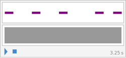
Here we generate the clave son (commonly just called clave) rhythm, a central facet of any salsa dance:
In[2]:=
EmitSound[Sound[{SoundNote["Clap",0.75],SoundNote["Clap",0.75],SoundNote["Clap",1.0],SoundNote["Clap",0.5],SoundNote["Clap",1.0]}]]
Sound familiar? That pattern is the foundation of nearly all Afro-Cuban music. Usually, it’s played on an instrument called claves which are two cylindrical pieces of resonant hardwood that produce a sound that cuts through the entire ensemble to communicate this pattern as a foundation to the music that’s going on around it.
◼
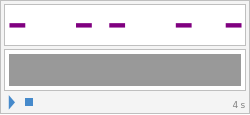
The same rhythm, but this time with a claves sound instead of clapping. Here, we use a pure function to avoid retyping our instrument name each time:
In[3]:=
EmitSound[Sound[{SoundNote[#,0.75],SoundNote[#,0.75],SoundNote[#,1.0],SoundNote[#,0.5],SoundNote[#,1.0]}]]&["Claves"]
Interestingly enough, this is same pattern is also known in rock and roll music as the “Bo Diddley beat,” named after rhythm and blues musician Bo Diddley.
◼
Again, we have the same timeline, now with a bass drum:
In[4]:=
EmitSound[Sound[{SoundNote[#,0.75],SoundNote[#,0.75],SoundNote[#,1.0],SoundNote[#,0.5],SoundNote[#,1.0]}]]&["BassDrum"]
Up until now, we’ve been generating these timelines by creating a sequence of SoundNotes with pre-determined lengths in seconds (take a look at the second argument of each SoundNote). However, in music we hear what many call a “pulse” or the thing you tap your foot to. The pulse is just a set of identical, repeated, and periodic stimuli.
◼
Here’s a steady pulse (repeated 16 times) every 0.25 seconds:
In[7]:=
EmitSound[Sound[Table[SoundNote[#,0.25],16]]]&["Clap"]
So if every rhythm is built off of this pulse, can we express our earlier clave rhythm in terms of this pulse? Of course! Let’s assume a pulse with a duration of 0.25. That means that each hit or onset will be a minimum of 0.25 seconds away from each other.
EmitSound[Sound[{SoundNote[#1,#2*3],SoundNote[#1,#2*3],SoundNote[#1,#2*4],SoundNote[#1,#2*2],SoundNote[#1,#2*4]}]]&["Claves",0.25]
So in that case, we’re expressing each onset as a certain multiple of our base pulse of 0.25. Because we’re dealing with percussion instruments, we could also just express every single pulse, with some being silent.
◼
To “play” silence, we use an Instrument called None:
EmitSound[Sound[{SoundNote[#1,#2],SoundNote[None,#2],SoundNote[None,#2],SoundNote[#1,#2],SoundNote[None,#2],SoundNote[None,#2],SoundNote[#1,#2],SoundNote[None,#2],SoundNote[None,#2],SoundNote[None,#2],SoundNote[#1,#2],SoundNote[None,#2],SoundNote[#1,#2],SoundNote[None,#2],SoundNote[None,#2],SoundNote[None,#2]}]]&["Claves",0.25]
The last thing we need to talk about is tempo. Tempo, in music, is just the speed of the pulse, usually measured in beats per minute. Well, in our previous example, we had 0.25 seconds per beat, so how do we find the number of beats per minute for that particular pulse length?
In[13]:=
Out[13]=
We can also reverse this process. That is, given a tempo, we can calculate how long each pulse is in seconds.
In[23]:=
Out[23]=
Visualization
Visualization
Up until now, we’ve just been listening to patterns without any way of visualizing the rhythms we’ve been playing with. But remember, our rhythms are just sequences of periodic pulses! So why not just represent each pulse by a square?
◼
Here, we use the ArrayPlot function to plot an array of 16 0s:
In[36]:=
ArrayPlot[{Table[0,16]},MeshAll]
Out[36]=
With percussion instruments we only have onsets (hits) and rests, so we can just represent an onset as a filled in square while a rest is a blank square. If each square is 0.25 seconds in length, then to recreate our clave pattern, we need to fill in the 1st, 4th, 7th, 11th, 13th boxes.
◼
We create the same diagram, but this time we add in onsets by using 1s (we also play the rhythm):
In[151]:=
ArrayPlot[{{1,0,0,1,0,0,1,0,0,0,1,0,1,0,0,0}},MeshAll]EmitSound[Sound[{SoundNote[#1,#2*3],SoundNote[#1,#2*3],SoundNote[#1,#2*4],SoundNote[#1,#2*2],SoundNote[#1,#2*4]}]]&["Claves",0.25]
Out[151]=
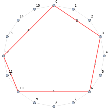
Remember that these rhythmic timelines are cyclic: you reach the end and cycle back to the beginning. So another way to represent these would be to use a circular structure like a binary necklace.
◼
Here we have the pulse represented by points on a circle and our pattern is represented by the nodes connected by the red edges (we use 0-indexed pulses because that’s how music theorists do it:
In[139]:=
Graph[Reverse[Range[0,15]],Join[Property[#,EdgeStyle{Black,Thin}]&/@Table[i<->Mod[i+1,16],{i,0,15}],Property[#,EdgeStyle{Red,Thick}]&/@{03,36,6<->10,10<->12,120}],GraphLayout"CircularEmbedding",VertexLabelsAll,EdgeLabels{033,363,6<->104,10<->122,1204}]
Out[139]=
In[95]:=
Checkout the shape formed by the pattern in our cyclic representation. Maybe humans find rhythms with irregular polygon shapes more interesting than those with regular polygon representations... We won’t explore that idea here, but maybe try it on your own!
We’ll focus on the first type of visualization, often called a TUBS (Time Unit Box System) diagram for the rest of our exploring.
We’ll focus on the first type of visualization, often called a TUBS (Time Unit Box System) diagram for the rest of our exploring.
Generation
Generation
An interesting consequence of our TUBS diagram is any easy to extract binary representation of our rhythm. It’s simple: 0 is a rest and a 1 is an onset. In fact, if we take a look at our earlier TUBS generation code, that’s exactly how we gave ArrayPlot our rhythmic pattern!
In[161]:=
ArrayPlot[{{1,0,0,1,0,0,1,0,0,0,1,0,1,0,0,0}},MeshAll]
Out[161]=
Of course, we also need a way to actually sonify this new way of representing our rhythms. Below, we write a function that takes in two arguments, a binary array and a tempo, and creates a Sound that we can hear.
In[1]:=
sonifyRhythm[instrument_, pattern_, tempo_]:= Sound[SoundNote[#, (tempo/60)^-1]& /@ (pattern /. {0 None, 1 instrument})]
Having this binary form of our rhythm means we can easily do computations on it without leaving our pulse-based system.
◼
Rotate (shift beats):
In[258]:=
clave={1,0,0,1,0,0,1,0,0,0,1,0,1,0,0,0}ArrayPlot[{clave},MeshAll,PlotLabel"clave"]sonifyRhythm["Claves",clave,240.0]ArrayPlot[{RotateLeft[clave,4]},MeshAll,PlotLabel"RotateLeft[clave, 4]"]sonifyRhythm["Claves",RotateLeft[clave,4],240.0]ArrayPlot[{RotateRight[clave,4]},MeshAll,PlotLabel"RotateRight[clave, 4]"]sonifyRhythm["Claves",RotateRight[clave,4],240.0]
Out[258]=
{1,0,0,1,0,0,1,0,0,0,1,0,1,0,0,0}
Out[259]=
Out[260]=
Out[261]=
Out[262]=
Out[263]=
◼
Invert:
In fact, these are common rules that musicians and composers use to change up rhythms in real music.
We could get even fancier by generating a new rhythm after each playthrough by using 1-D cellular automata rules.
We could get even fancier by generating a new rhythm after each playthrough by using 1-D cellular automata rules.
◼
Using rule 30 (the top row is the first generation, the 2nd row the second generation, and so forth):
Bonus: Cross beats
Bonus: Cross beats
In complex pieces of music, particularly Jazz, musicians often like to create “rhythmic complexity” by creating polyrhythms. We didn’t get a chance to explore the idea of macro-beats in our previous explorations, but suffice it to say for now that often times we hear groupings of pulses instead of a the lowest common micro-pulse. It’s this macro-beat that we usually end up tapping our foot to. The cool thing about these macro-pulses is that they can be made up of different numbers of micro-pulses based on the music you’re playing. This leads to a concept of rhythmic meter which we don’t have time to explore in-depth. Instead, let’s talk about “cross beats” which rely on the ear hearing a simultaneous expression of two different kinds of macro beats.
Pretend you’re a drummer from Ghana. You’re given 20 micro-pulses and asked to play on the first of the 20 pulses and four other evenly spaced pulses. In other words, you have five evenly spaced onsets.
Now do the same thing, except you need to play on 3 other evenly spaced pulses. In other words, you have four evenly spaced onsets.
If these two players were to play at the same time, the human ear (and brain) senses the tension between the two different rhythmic sub divisions. This is a really common technique in West African drum music.
◼
Here we have one drummer play 4 evenly space hits while the other plays 5 evenly spaced hits (these are grouped together into one instrument for simplicity):
Things we didn’t get to
Things we didn’t get to
We’ve barely scratched the surface of musical rhythm. This was just meant as an intro to seeing how we could formally express, visualize, and generate new rhythms using the Wolfram Language. A great next step would be to explore musical meter, a concept that lots of beginning musicians have trouble with.
Further Explorations
Musical Geometry
Musical Structure (Voice Leading and Part Writing)
Classical Fugue Analysis
Composing from the Greats: Using Machine Learning to Generate Musical Compositions
Musical Structure (Voice Leading and Part Writing)
Classical Fugue Analysis
Composing from the Greats: Using Machine Learning to Generate Musical Compositions
Authorship information
Connor Bain
June 23, 2017 - v1.1
connorbain@u.northwestern.edu


