Riemann Sum
Riemann Sum
Approximating the definite integral
Explanation
Explanation
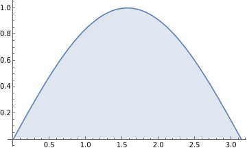
Let’s suppose you want to obtain the area under the curve in a plot
◼
Example curve and area
In[42]:=
area = NIntegrate[Sin[x], {x, 0, Pi}];Grid[{{functionPlot :=Plot[Sin[x], {x, 0, Pi}, FillingAxis, ImageSizeMedium]; functionPlot},{"Actual area: " <> ToString[area//N]}}]
Out[43]=
Actual area: 2. |
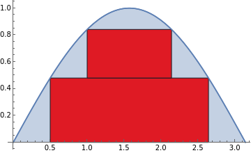
If you were drawing the curve in paper, it is not really possible to measure it directly as it is. The most naive approach is to draw geometrical figures to which is know how to calculate their area. For example, rectangles.
◼
Representing the curve as rectangles
In[37]:=
rectCoord = {{{0.5,0},{Pi-0.5,0},{Pi-0.5, Sin[0.5]},{0.5,Sin[0.5]}},{{1.0, Sin[0.5]},{Pi-1,Sin[0.5]},{Pi-1,Sin[1]},{1,Sin[1]}}};bars =Map[ Graphics[ EdgeForm[{Thickness[Medium], Black}], Red, Polygon[#]]&,rectCoord];rectArea = Plus @@ Map[Area @ Polygon[#]&, rectCoord];error := Abs[area-rectArea];Grid[{{Show[Flatten[{functionPlot, bars, functionPlot}], ImageSize->Medium]},{"Rectangle area " <> ToString[rectArea // N]},{"Actual area " <> ToString[area // N]},{"Error " <> ToString[error // N]}}]
Out[41]=
Rectangle area 1.44004 |
Actual area 2. |
Error 0.559957 |
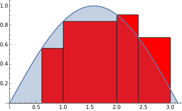
We can simplify our approximation making rectangle’s height be dependant of the curve’s values, for example
◼
Now the rectangle height depends on the curve height
In[33]:=
rectXCoord = {0,0.6}, {0.6,1}, {1,2}, {2,2.4}, {2.4, 3};bars =Map[ Graphics[ EdgeForm[{Thickness[Medium], Black}], Red, Polygon[{{#[[1]],0},{#[[2]],0},{#[[2]], Sin[#[[1]]]},{#[[1]], Sin[#[[1]]]}}]]&,rectXCoord];rectArea = Plus @@ Map[ (#[[2]] - #[[1]]) * Sin[#[[1]]]&, rectXCoord];Grid[ {Show[Flatten[{functionPlot, bars, functionPlot}],ImageSizeMedium]}, {"Rectangle area " <> ToString[rectArea // N]}, {"Actual area " <> ToString[area // N]}, {"Error " <> ToString[error // N]}]
Out[36]=
Rectangle area 1.83632 |
Actual area 2. |
Error 0.163675 |
In this example, the height is equal to the value of the function in the x value of the left-most side of the rectangle. The total area of the rectangles with this approach is:f()*(-)where the elements in X contain the positions of the left-most and right-most sides of each rectangleTo make or approximation even more simple to calculate, we can make all rectangles to have the same width and to assure all rectangles are adjacent with each other
∑
x∈X
x
Left
x
Right
x
Left
In[21]:=
(*Obtains the area of all rectangles in the Riemann sum*)riemannArea [function_, start_, end_, rectNumber_, type_String:"Left"]:= Plus @@ Table (end - start) rectNumber * Switch type, "Left", function[x], "Right", function[x + (end - start) / rectNumber], "Mean", (function[x] + function[x + (end - start) / rectNumber]) 2.0 , {x, start, end - (end - start) / rectNumber, (end - start) / rectNumber};
In[13]:=
(*Draws the plot and rectangles for the Riemann sum*)riemannGraphic[function_, start_, end_, rectNumber_Integer, type_String:"Left"] := Show RectangleChart Table (end - start) rectNumber, Switch type, "Left", function[x], "Right", function[x + (end - start) / rectNumber], "Mean", (function[x] + function[x + (end - start) / rectNumber]) 2.0 , {x, start, end - (end - start) / rectNumber, (end - start) / rectNumber} , BarSpacingNone, ChartStyleRed, ImageSizeMedium , Plot[function[x], {x, start, end}, FillingAxis, ImageSizeMedium];
◼
Covering the curve with rectangles of the same width
Approaching the error to zero
There are many parts of the curve that are still not covered by the rectangles, this can improve if we use more rectangles of smaller size
◼
Trying with a smaller rectangle width
The rectangle height doesn’t necessarily have to be the value of the curve on the left side, it can also use the right side or the mean of both. These are the most common methods.
◼
Showing a graph with variable rectangle quantity and method and calculating the total area of the rectangles, the curve and comparing their difference
As you can see, the more rectangles you add, the lesser the error is. In fact the error tends to zero as the number of rectangles of equal width tend to infinite.
◼
Plot to the error given the number of rectangles
Given how the Riemann sum converges with the area under a curve, it is useful as an approximation for the definite integral.
Further Explorations
Definite integral
Lebesgue integration
Authorship information
Itzel Carolina Delgadillo Perez
June 22nd 2017
caroagsmex@hotmail.com