Linear Regression with Outliers
Linear Regression with Outliers
Linear regression based on minimizing squared distances does not work well when some of the data points are outliers, meaning points far away from a presumptive well-fitting line. We discuss an easy modification that allows linear regression to work well even in the presence of outliers.
Utilities
Utilities
◼
Utilities to plot a function and to plot a list of points:
In[1]:=
functionPlot[fn_,style_]:=Block[{x},Plot[fn[x],{x,0,7},PlotStyle->style]]listPlot[list_,style_]:=ListPlot[list,PlotStyle->style]
◼
Utility to compute the slope and intercept of the linear function through two points:
In[3]:=
twoPointLine[{{x1_,y1_},{x2_,y2_}}]:=Module{slope,intcpt}, slope=Ifx2-x1≠0,,0,intcp=y1-slope*x1
y2-y1
x2-x1
Standard Least Squares
Standard Least Squares
Classical Least Squares fits a straight line to a set of data points by minimizing the sum of the squared vertical distances. We’ll demonstrate this with an example.
◼
First generate a set of “inlier” points near a fixed straight line:
In[4]:=
Clear[x];linf[x_]=0.5*x+1.0;inlierPoints=Table[{x,linf[x]+RandomReal[{-0.2,0.2}]},{x,1,6}];Show[listPlot[inlierPoints,{Gray,PointSize[0.02]}],functionPlot[linf,{Gray,Dotted}]]
Out[7]=
◼
The (solid red) line that minimizes the sum of squared vertical distances to each of the inlier points is close to the original (gray dotted) line:
In[8]:=
pointSet=inlierPoints;Clear[a,b,x,f,xp,yp]{xp,yp}=Transpose[pointSet];n=Length[pointSet];f[x_]=b*x+a;objective=;fitLine[x_]=a+bx/.Last[Minimize[objective,{a,b}]]Show[listPlot[pointSet,{Gray,PointSize[0.02]}],functionPlot[linf,{Gray,Dotted}],functionPlot[fitLine,Hue[1.0]]]
n
∑
i=1
2
(Indexed[yp,i]-f[Indexed[xp,i]])
Out[14]=
1.03039+0.503843x
Out[15]=
But including a few “outlier” points that are far away from the original can have large unwanted effects on the fitted line.
◼
Least squares minimization now gives a line (blue) that is not near the original gray line:
In[16]:=
outlierPoints={{1.5,4},{5.5,1}};mixedPoints=Join[outlierPoints,inlierPoints];pointSet=mixedPoints;Clear[a,b,x,f,xp,yp]{xp,yp}=Transpose[pointSet];n=Length[pointSet];f[x_]=b*x+a;objective=;fitLine[x_]=a+bx/.Last[Minimize[objective,{a,b}]]Show[listPlot[pointSet,{Gray,PointSize[0.02]}],functionPlot[linf,{Gray,Dotted}],functionPlot[fitLine,Hue[0.65]]]
n
∑
i=1
2
(Indexed[yp,i]-f[Indexed[xp,i]])
Out[24]=
2.3337+0.110481x
Out[25]=
Modifying Least Squares to handle outliers
Modifying Least Squares to handle outliers
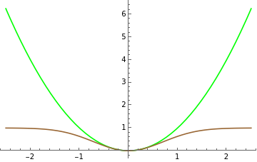
Outliers have a big effect on least squares because the quadratic function applied to each deviation grows very quickly as the argument moves away from zero. We will replace the quadratic function by an (inverted and shifted) gaussian function that behaves similarly for small values of the argument, but that does not grow very much for larger values of the argument.
◼
The quadratic function is displayed in green, the (inverted and shifted) gaussian function is displayed in brown:
In[26]:=
quadratic[x_]=;gaussian[x_]=1-Exp[-];Plot[{quadratic[x],gaussian[x]},{x,-2.5,2.5},PlotStyle{Green,Brown}]
2
x
2
x
Out[28]=
For the set consisting of only inlier points, the modification produces a line (red) close to the original gray line.
This is similar to the result of the unmodified Least Squares fit:
This is similar to the result of the unmodified Least Squares fit:
◼
Perform the modified Least Squares fit on the inlier set:
In[29]:=
pointSet=inlierPoints;Clear[a,b,x,f,xp,yp]{xp,yp}=Transpose[pointSet];n=Length[pointSet];f[x_]=b*x+a;objective=gaussian[Indexed[yp,i]-f[Indexed[xp,i]]];fitLine[x_]=a+bx/.Last[Minimize[objective,{a,b}]]Show[listPlot[pointSet,{Gray,PointSize[0.02]}],functionPlot[linf,{Gray,Dotted}],functionPlot[fitLine,Hue[1.0]]]
n
∑
i=1
But while the unmodified Least Squares fit performed poorly when outliers were included, the modified fit essentially ignores the outlier and still provides a good fit to the original line.
◼
Perform the modified Least Squares fit on the set containing both inlier and outliers, and also record the minimum value of the cost function:
Behind the scenes
Behind the scenes
There is a price to pay in increasing the complexity of the function for the two-parameter minimization. In particular, while the standard least squares minimizes a function with a unique local minimum, the modified procedure minimizes a function that may have several distinct local minima:
◼
Display contour plots for the objective functions that occur in classical version, and in the modified version:
The sophisticated “Minimize” function was able to find the global minimum even when there a multiple local minima.
A less sophisticated gradient flow minimization depends on initial conditions, and still works well in the simpler traditional case. But for the modified case, a local minimum can trap the gradient flow and prevent it from finding a global minimum, as shown with the series of examples below:
A less sophisticated gradient flow minimization depends on initial conditions, and still works well in the simpler traditional case. But for the modified case, a local minimum can trap the gradient flow and prevent it from finding a global minimum, as shown with the series of examples below:
◼
Compute a gradient flow minimization starting with the dotted colored line connecting two outlier points. The solid colored line is the result of the gradient flow minimization, and it is a very poor fit to the initial gray dotted line:
◼
Compute a gradient flow minimization starting with the dotted colored line connecting two inlier points. The solid colored line is the result of the gradient flow minimization, and it finds the correct global minimum.
RANSAC (RAndom SAmple Consensus) is a method for choosing good initial conditions for gradient fit, without knowledge of which points are inliers and which points are outliers. A pair of data points is randomly chosen, and the cost function is computed for the line passing through the two points. This process is repeated several times, and the pair with the lowest cost function is chosen as the initial condition. The initial conditions chosen this way are likely to be near the global minimum, so gradient flow is likely to find the correct global minimum rather than being trapped at a local minimum.
◼
The following graph illustrates RANSAC. Each colored dotted line passes through two data points. The color coding of each dotted lines indicates cost of the line, the red lines being good starting points for a gradient flow optimization.
Further Explorations
Random Sample Consensus (RANSAC)
Hough Transform
Authorship information
Jan Segert
June 21, 2017
segertj@gmail.com
