Monte Carlo Integration
Monte Carlo Integration
Approximating definite integrals with random sampling
Principles and Motivation
Principles and Motivation
The integral of the Gaussian function is famously inexpressible in terms of elementary functions. Yet, there are many situations (e.g. when computing normalising constants of distributions in statistics) in which the definite integrals of such functions appear, and must be computed numerically.
◼
Define the Gaussian function:
In[9]:=
gaussianFunction[x_]=Exp[-x^2]
Out[9]=
-
2
x
◼
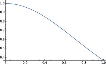
Plot the Gaussian function on the interval [0,1]:
In[10]:=
gaussianPlot=Plot[gaussianFunction[x],{x,0,1}]
Out[10]=
When definite integrals cannot be evaluated analytically, one approach to evaluating them numerically (assuming that the range of the integrand is bounded) is to treat the limits of integration, and the local maximum and minimum of the function within that region, as the edges of a rectangle. Then, one places random points inside that rectangle using uniform sampling.
◼
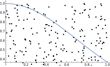
Pick a set of 250 random points to place on the Gaussian function plot above.
In[20]:=
randomPoints=RandomPoint[Rectangle[],250];
◼
Add the random points to the Gaussian plot:
In[21]:=
Show[gaussianPlot,Graphics[Point[randomPoints]]]
Out[21]=
Clearly, the probability of any such a point being enclosed between the function and the y-axis is equal to the ratio of the area enclosed by the function to the total area of the rectangle. Thus, the ratio of the number of points enclosed by the function to the total number of points, when multiplied by the area of the rectangle (which, in this case, is 1), gives an approximation to the value of the definite integral.
Approximating the Gaussian Integral
Approximating the Gaussian Integral
A point is enclosed by the function if its y-coordinate is less than or equal to the value of the function at its respective x-coordinate (since, in this case, the function is strictly non-negative). Conversely, a point is not enclosed by the function if its y-coordinate is strictly greater than the value of the function at its respective x-coordinate.
◼
Determine the set of points enclosed by the Gaussian function:
In[34]:=
insidePoints=Cases[randomPoints,{x_,y_}/;y≤gaussianFunction[x]];
◼
Determine the set of points that lie outside the Gaussian function:
In[35]:=
outsidePoints=Cases[randomPoints,{x_,y_}/;y>gaussianFunction[x]];
◼
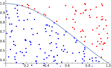
Show the points enclosed by the Gaussian function in blue, and all others in red:
In[36]:=
Show[gaussianPlot,Graphics[{Red,Point[outsidePoints]}],Graphics[{Blue,Point[insidePoints]}]]
Out[36]=
The fraction of the points enclosed by the function provides an approximation of the value of the definite integral. The more points that are placed, the better the approximation.
◼
Approximate the value of the Gaussian integral:
In[27]:=
value=Length[insidePoints]/Length[randomPoints]
Out[27]=
94
125
◼
Compute the absolute error (i.e. the difference between this crude numerical approximation, and Mathematica’s own numerical approximation):
In[28]:=
Abs[value-NIntegrate[Exp[-x^2],{x,0,1}]]
Out[28]=
0.00517587
This method of uniform sampling is known as ‘naive’ Monte Carlo integration.
Higher-Dimensional Generalisation
Higher-Dimensional Generalisation
In practice, one-dimensional integrals can be approximated much more efficiently (except in highly pathological cases) by using interpolating functions as quadrature rules. A good example is given by the Newton-Cotes formulae, which approximate a function by interpolating between polynomials placed at equally spaced points. As such, Monte Carlo methods are usually only practical when evaluating integrals in many dimensions, since (unlike interpolation methods) the technique generalises naturally to spaces of arbitrary dimensionality.
◼
Generalise the Gaussian function to 2 dimensions:
In[52]:=
gaussianFunction2[x_,y_]=Exp[-(x^2+y^2)]
Out[52]=
--
2
x
2
y
◼
Plot the 2-dimensional Gaussian inside a box of volume 1:
In[54]:=
gaussianPlot2=Plot3D[gaussianFunction2[x,y],{x,0,1},{y,0,1}]
Out[54]=
Now, we generalise the Monte Carlo procedure by sampling uniformly inside the space, and determining which points are enclosed by the surface.
◼
Pick a set of 10,000 random points to place inside the space:
In[55]:=
randomPoints2=RandomPoint[Cuboid[],10000];
◼
Determine the set of points enclosed by the Gaussian surface:
In[57]:=
insidePoints2=Cases[randomPoints2,{x_,y_,z_}/;z≤gaussianFunction2[x,y]];
◼
Determine the set of points that lie outside the Gaussian surface:
In[58]:=
outsidePoints2=Cases[randomPoints2,{x_,y_,z_}/;z>gaussianFunction2[x,y]];
◼
Show the points enclosed by the Gaussian surface in blue, and all others in red:
In[59]:=
Show[gaussianPlot2,Graphics3D[{Red,Point[outsidePoints2]}],Graphics3D[{Blue,Point[insidePoints2]}]]
Out[59]=
Once again, we obtain an asymptotic approximation to the value of the (higher-dimensional) integral.
◼
Approximate the value of the higher-dimensional integral:
In[60]:=
value2=Length[insidePoints2]/Length[randomPoints2]
Out[60]=
5561
10000
◼
Compare with Mathematica’s approximation:
In[61]:=
Abs[value2-NIntegrate[Exp[-(x^2+y^2)],{x,0,1},{y,0,1}]]
Out[61]=
0.0016463
Many improvements can be made to the uniform sampling approach used in naive Monte Carlo integration. For instance, the target area may be split into several sub-domains that are each sampled separately (known as ‘stratified sampling’), a non-uniform sampling distribution may be used (known as ‘importance sampling’), and so on. When employed correctly, such approaches can dramatically reduce the standard error of the approximation by increasing its convergence time. Finding improved estimates for the error in Monte Carlo techniques remains an active area of research.
Further Explorations
Stratified sampling
Importance sampling
Mean field particle methods
Umbrella sampling (computational physics)
Authorship information
Jonathan Gorard
06/21/17
jonathan.gorard@kcl.ac.uk


