Modelling a Submarine Using Potential Flow Analysis
Modelling a Submarine Using Potential Flow Analysis
Potential flow analysis can be used to model a variety of objects, and how they interact with fluid flows.
Uniform Flow
Uniform Flow
The most basic potential flow regime is a uniform stream in the x direction.
◼
Let’s model a stream with velocity U=5:
In[6]:=
U=5;
◼
The following are the stream function and velocity potential, respectively:
In[7]:=
ψuniform[y_]=Uy;ϕuniform[x_]=Ux;
Finding the x and y components of the velocity is trivial in this case, but it will help with understanding a more complex flow later.
◼
To find the x component of the velocity of the stream, we take the derivative of the velocity potential with respect to x:
In[9]:=
u=D[ϕuniform[x],x]
Out[9]=
5
◼
To find the y component, we take the negative derivative of the stream function with respect to y:
In[10]:=
v=-D[ψuniform[x],y]
Out[10]=
0
◼
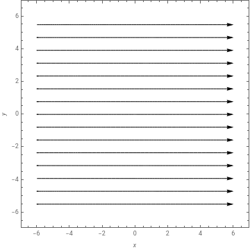
Now let’s plot the stream lines of the flow:
In[11]:=
StreamPlot[{u,v},{x,-6,6},{y,-6,6},StreamScaleFull,FrameLabel{x,y},StreamStyle{Arrowheads[.03],Black}]
Out[11]=
Source or Sink at the Origin
Source or Sink at the Origin
The next potential flow regime we will need is a source (or sink) at the origin. In either case, the z axis is treated as an infinitesimally thin pipe manifold, through which fluid is ejected (or sucked in) at volume flow rate Q that is uniform along its length b.
◼
Let’s model a source at the origin with the following values for volume flow rate and length:
In[12]:=
Q=2000;b=200;
◼
The source will have strength m, defined by:
In[14]:=
m=;
Q
2πb
◼
At a given position (x,y), the velocity potential will be:
In[15]:=
ϕsource[x_,y_]=mLog+;
2
x
2
y
◼
and the stream function will be:
In[16]:=
ψsource[x_,y_]=mArcTan;
y
x
◼
From here, we can find the x and y velocity components via derivation:
In[17]:=
[x_,y_]=D[ψsource[x,y],y];[x_,y_]=D[ϕsource[x,y],y];
◼
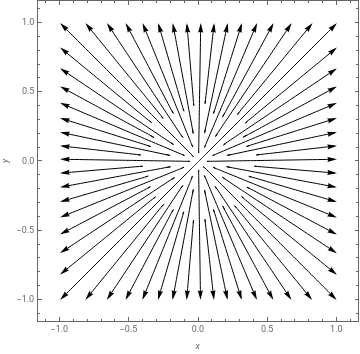
Let us now make a plot of the stream lines:
In[19]:=
StreamPlot[{[x,y],[x,y]},{x,-1,1},{y,-1,1},StreamScaleFull,FrameLabel{x,y},StreamStyle{Arrowheads[.03],Black}]
Out[19]=
Rankine Half-Body
Rankine Half-Body
A good way to model a submarine moving through water is to approximate the submarine as a Rankine half-body shape. This is the shape that occurs when a uniform flow encounters a single source. We can use our uniform flow and source from above.
◼
We first define the x velocity component by adding together the x velocity components for the uniform stream and source:
In[20]:=
[x_,y_]=u+[x,y];
◼
Likewise, we define the y velocity component by adding together the y velocity components for the uniform stream and source:
In[21]:=
[x_,y_]=v+[x,y];
◼
Before plotting the streamlines, we should make a list of points that we want the streamlines to go through:
In[22]:=
points=
;
-0.5 | -0.5 |
-0.5 | 0 |
-0.5 | 0.5 |
-0.25 | -0.5 |
-.25 | 0 |
-0.25 | 0.5 |
0 | -0.5 |
0 | 0 |
0 | 0.25 |
0 | -.25 |
0 | 0.5 |
.25 | -.5 |
0.25 | -0.25 |
0.25 | 0 |
0.25 | 0.25 |
0.25 | 0.5 |
0.5 | -0.5 |
0.5 | 0 |
0.5 | 0.5 |
-.25 | .25 |
-.25 | -.25 |
◼
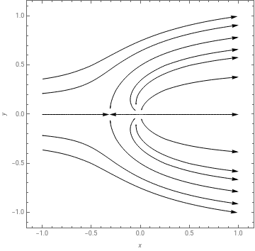
Now, let’s plot the streamlines:
In[23]:=
StreamPlot[{[x,y],[x,y]},{x,-1,1},{y,-1,1},StreamScaleFull,FrameLabel{x,y},StreamStyle{Arrowheads[.03],Black},StreamPointspoints]
Out[23]=
As we can see, the streamlines form a roughly elliptical half-body shape. At the nose of the body is a stagnation point, where the flow velocity is zero. This shape represents the upstream end of our submarine moving through the water.
◼
To make the visualization even more clear, we can omit the streamlines that are “inside” the submarine by specifying new points for the streamlines to go through:
◼
Our new plot shows only the streamlines defining the nose of the submarine, and the water passing around it:
Further Explorations
Try modeling a symmetrical airfoil using a series of sinks and sources in a uniform flow
Try modeling an airfoil in a uniform stream near the ground by using an image airfoil
Authorship information
Kaleb Alekel
6-21-17
ka5@geneseo.edu


