An Introduction to Markov Chains

A Markov chain is a series of random variables, known as states, that satisfy the Markov Property: the probability of the current state only depends on the state that preceded it. In other words, past and future states are stochastically independent. The “time” can be discrete, continuous, or more generally, a totally ordered set.

Example of Markov Chains

A mouse in a cage with two cells 1 and 2 containing fresh and stinky cheese. The mouse is in cell 1 at time n, then at time n + 1 it is either still in 1 or has moved to 2. Statistical observation shows that the mouse moves from cell 1 to cell 2 with probability α = 0.05 regardless of where it was at earlier times. Similarly it moves from 2 to 1 with probability β = 0.99. This can be represented by a transition diagram, and/or a transition probability matrix.

transitionMatrix={{0.95,0.05},{0.99,0.01}};

g=Graph[DiscreteMarkovProcess[1,transitionMatrix]];Scan[(PropertyValue[{g,#},EdgeLabels]=PropertyValue[{g,#},"Probability"])&,EdgeList[g]];g

transitionMatrix//MatrixForm



0.95	0.05
0.99	0.01



Stationarity

When a Markov chain is stationary we refer to it as being in steady-state. A Markov chain is stationary if it starting with a stationary distribution, the marginal distribution of all states at any time will always be the stationary. Assuming irreducibility,if the stationary distribution exists, it is always unique, and its existence can be implied by positive recurrence of all states. Markov chains that exhibit this property are also called Regular Markov Chains.

Example

Assume there is a company A that currently owns 20% of the market; if certain advertising campaign is applied to A the probability of a customer of brand B switching to brand A is 60% and the probability of a customer of brand A keeping his/her loyalty to the brand is 80%.

Let’s see what happens:

initialState={{0.1,0.9}};prob={{0.8,0.2},{0.6,0.4}};initialState.prob

According to this operation, we see that brand A will own approximately 60% of the market after

. Now if we repeat this operation we’ll see this is a trend. However after

brand A’s market share will stop increasing and stays the same. This means this is a steady-state system with a stationary matrix.

mark[initial_,probM_,iter_]:=Module[{init=initial,prob=probM,it=iter},aList={};res=init;For[i=0,i<it,i++,res=res.prob;AppendTo[aList,res];];Return[aList]]

mark[initialState,prob,10]

{{{0.62,0.38}},{{0.724,0.276}},{{0.7448,0.2552}},{{0.74896,0.25104}},{{0.749792,0.250208}},{{0.749958,0.250042}},{{0.749992,0.250008}},{{0.749998,0.250002}},{{0.75,0.25}},{{0.75,0.25}}}

List[initialState,prob,10]

{{{0.1,0.9}},{{0.8,0.2},{0.6,0.4}},10}

Properties of Regular Markov Chains

Let P be the transition matrix for a regular Markov chain, now:

◼

There is a unique stationary matrix S that can be found by solving S×P = S

◼

Given any initial state matrix (

), the state matrices

approach the stationary matrix S.

◼

The matrices

approach a limiting matrix

, where each row of

is equal to the stationary matrix S.

Example

Find stationary matrix for P,

P=MatrixForm[{{0.6,0.4},{0.2,0.8}}]



0.6	0.4
0.2	0.8



Putting S×P = S into equation form: [

].[

0.6	0.4
0.2	0.8

] =[

]Now, we can use a method like substitution, to solve for

and

s=Solve[0.6*(1-s2)+0.2*s2==1-s2]

Therefore our stationary matrix S = [

]

Absorbing Markov Chains

◼

A state in a Markov chain is called an absorbing state if once the state is entered it is imposable to leave.

◼

Like regular Markov chains, absorbing Markov chains have the property that the powers of the transition matrix approach a limiting matrix.

◼

The presence of an absorbing state in a transition matrix does NOT guarantee that the power of the matrix approach a limiting matrix nor that the state matrices in the corresponding Markov chain approach a stationary matrix.

◼

For transition matrices for Markov chains with one or more absorbing states to have liming matrices, we need to have an absorbing Markov chain. A Markov chain is an absorbing chain if:

◼

There is at least one absorbing state

◼

It is possible to go from each non-absorbing state to at least one absorbing state in a finite number of steps.

Example

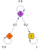
The following is an example represent an absorbing Markov chain given that it contains one absorbing state and you can go from 2 to 1 and from 3 to 1.

absorbing={{1,0,0},{.2,.8,0},{0,.1,.9}};proc=DiscreteMarkovProcess[1,absorbing];MarkovProcessProperties[proc,"AbsorbingClasses"]

g=Graph[proc];Scan[(PropertyValue[{g,#},EdgeLabels]=PropertyValue[{g,#},"Probability"])&,EdgeList[g]];g

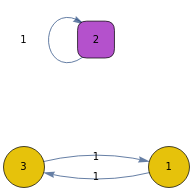
absorbing={{0,0,1},{0,1,0},{1,0,0}};proc=DiscreteMarkovProcess[1,absorbing];MarkovProcessProperties[proc,"AbsorbingClasses"]

The following is an example is not an absorbing Markov chain given that although it contains one absorbing state it is not possible to go from each non-absorbing state to the absorbing state

g=Graph[proc];Scan[(PropertyValue[{g,#},EdgeLabels]=PropertyValue[{g,#},"Probability"])&,EdgeList[g]];g

Random Walk

A special kind of of Markov Chains known as a Random Walk, is a chain that presents spatial homogeneity in addition of time-homogeneous transition probabilities. In other words, at every state, the next step is an outgoing edge chosen according to an arbitrary distribution.

A simple random walk is symmetric if the the moving “object” has the same probability for each of it’s neighbors.

Let’s define a better function to simulate Markov chains. simulateMChain, simulates a chain of length n with initial distribution

and transition distribution p. Here p is a function returning the probabilities

i,j1

,...

i,jk

where j represent the states that belong to S that can be reached in one step from state i in S.

simulateMChain[p0_,p_,n_]:=Module[{init=p0,transP=p,chainL=n},chain=ConstantArray[RandomChoice[init],chainL+1];For[i=1,i≤chainL,i++,chain[[i+1]]=RandomChoice[transP[chain[[i]]]]];Return[chain[[2;;]]];]

Simple Symmetric Random Walk

Bounded Symmetric Random Walk

The following is a simulation of a random walk using absorbing barriers between -10 and 10. As explained above, if the walk reaches any of these states, it will stay there. This example uses the same transition distribution as before. This time however let’s start all walks in 0.

Asymmetric Random Walk

The following graph represents a random walk where the initial distribution is asymmetric. Notice that even a slight change in probability drastically changes the general tendency of the trajectories.

Reluctant Random Walk

If a transition probability depends on the current position, the random walk is called reluctant. This is represented in the following graph. The closer we get to 0 or 10, the probability that any of these numbers are going to be reaches decreases. Thus we say the random walk is reluctant to end.