Benford’s Law
Benford’s Law
Benford’s Law is an empirical law in statistics that states that the leading significant digit of numerical data in real life is likely to be small.
Discovering Benford’s Law
Discovering Benford’s Law
In statistics, not a lot of attention is paid to the first digits of numbers. They seem so simple that it’s meaningless to study them.
◼
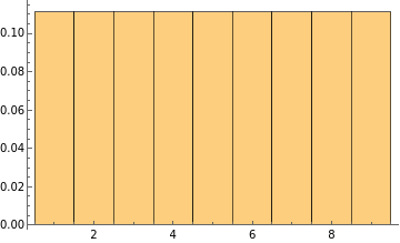
Make a histogram of the first digits of the first n natural numbers with n ranging from 10000 to 100000:
In[1]:=
Manipulate[Histogram[Array[IntegerDigits[#][[1]]&,n],9,"Probability"],{n,10000,100000,1000}]
Out[1]=
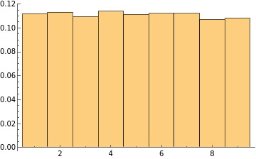
The pattern may look unfamiliar, but it’s easily understandable. Obviously, random integers behave similarly.
◼
Make a histogram of the first digits of 10000 random integers up to n with n ranging from 10000 to 100000:
In[2]:=
Manipulate[Histogram[DeleteCases[Table[IntegerDigits[RandomInteger[n]][[1]],10000],0],9,"Probability"],{n,10000,100000,1000}]
Out[2]=
This seems like a boring topic. Let’s take a look at some meaningful sequences, starting from the primes.
◼
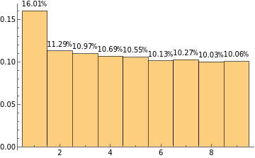
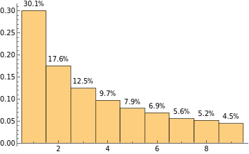
Make a histogram of the first digits of the first n primes with n ranging from 10000 to 100000:
In[3]:=
Manipulate[Histogram[Array[IntegerDigits[Prime[#]][[1]]&,n],9,"Probability",LabelingFunction(Placed[Row[{Round[100#,0.01],"%"}],Above]&)],{n,10000,100000,1000}]
Out[3]=
It seems that the first digit of primes is slightly more likely to be small, but the difference is nonobvious. But what about the Fibonacci numbers?
◼
Make a histogram of the first digits of the first n Fibonacci numbers with n ranging from 1000 to 10000:
In[4]:=
Manipulate[Histogram[Array[IntegerDigits[Fibonacci[#]][[1]]&,n],9,"Probability",LabelingFunction(Placed[Row[{Round[100#,0.01],"%"}],Above]&)],{n,1000,10000,100}]
Out[4]=
Whoa, wait a sec. Why is this so stable and what is this weird pattern? Let’s try more, say factorials.
◼
Make a histogram of the first digits of the first n factorials with n ranging from 100 to 1000:
In[5]:=
Manipulate[Histogram[Array[IntegerDigits[#!][[1]]&,n],9,"Probability",LabelingFunction(Placed[Row[{Round[100#,0.01],"%"}],Above]&)],{n,100,1000,10}]
Out[5]=
The same stable pattern shows again. This is getting interesting. What about powers of 2?
◼
Make a histogram of the first digits of the first n powers of 2 with n ranging from 1000 to 10000:
In[6]:=
Manipulate[Histogram[Array[IntegerDigits[2^#][[1]]&,n],9,"Probability",LabelingFunction(Placed[Row[{Round[100#,0.01],"%"}],Above]&)],{n,1000,10000,100}]
Out[6]=
This is too good to be coincidence. And yet this is not the end of story. Now let’s move on to some data from real life, starting with the populations of countries.
◼
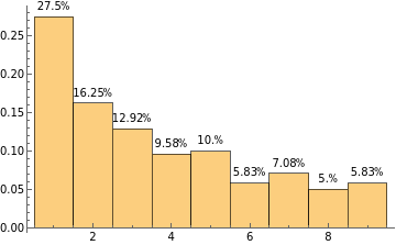
Make a histogram of the first digits of the populations of all the countries in the world:
In[7]:=
HistogramIntegerDigits[QuantityMagnitude[#]][[1]]&/@,9,"Probability",LabelingFunction(Placed[Row[{Round[100#,0.01],"%"}],Above]&),ImageSizeMedium
Out[7]=
The distribution is generally similar. What about the total areas of countries?
◼
Make a histogram of the first digits of the total areas of all the countries in the world in various units:
Does this pattern apply to any set of data? Let’s take a look at the heights of the tallest structures in the world.
◼
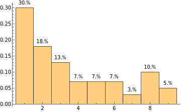
Make a histogram of the first digits of the heights of the top 1000 tallest structures in the world in various units:
Although the general trend holds in some histograms, most are quite divergent from the pattern that we saw above. The final example is the lengths of the longest rivers in the world.
◼
Make a histogram of the first digits of the lengths of the top 1000 longest rivers in the world in various units:
Curiously, the pattern seems to return. Is there a reason behind all this? The answer is Benford’s Law.
Introducing Benford’s Law
Introducing Benford’s Law
◼
The probability density function of Benford Distribution with base parameter 10:
◼
Plot a Benford Distribution:
It’s amazing how well the sequences of Fibonacci numbers, factorials, and powers of 2 fit Benford Distribution.
◼
Combine the plot of Benford Distribution and the histograms for the sequences of Fibonacci numbers, factorials, and powers of 2:
Many sets of data from real life also show good fit.
◼
Combine the plot of Benford Distribution with the histograms for populations, total areas, and lengths of rivers:
As we’ve seen above, there are exceptions that fit rather poorly.
◼
Combine the plot of Benford Distribution with the histograms for heights of structures:
A natural question is: why and when does Benford’s Law apply? Here’s a simple explanation.
Explaining Benford’s Law
Explaining Benford’s Law
◼
Plot a normal distribution with standard deviation 1/3 and the regions that correspond to numbers whose first digits are 1 and 9:
Since the data are very centralized and change rapidly in “blocks of 1”, they won’t obey Benford’s Law very well. On the other hand, what happens if a set of data has a broad distribution after taking log10?
◼
Plot a normal distribution with standard deviation 2 and the regions that correspond to numbers whose first digits are 1 (red) and 9 (blue):
Since the data are very flat in every “block of 1” and span several orders of magnitude rather uniformly, they will obey Benford’s Law very well.
This explains why the sequences of Fibonacci numbers, factorials, and powers of 2 obey Benford’s Law much better than the sequence of primes: the formers increase faster and therefore distribute more uniformly than the latter.
This explains why the sequences of Fibonacci numbers, factorials, and powers of 2 obey Benford’s Law much better than the sequence of primes: the formers increase faster and therefore distribute more uniformly than the latter.
◼
Plot the histograms of the sequences of Fibonacci numbers, factorials, powers of 2, and primes after taking log10:
Apparently, the first three histograms are very flat and uniform, while that of the prime sequence is unsymmetric and steep. The populations and total areas of countries are not as uniform, but they are rather symmetric and span several orders of magnitude.
◼
Plot the histograms of the populations and total areas of countries after taking log10:
On the other hand, since we take only the top 1000 tallest structures and there are many “tallish” buildings, the distribution is very narrow and unsymmetric as it’s greatly skewed to the right. The lengths of rivers are better because there are much fewer long rivers than tall buildings and the top 1000 longest rivers already includes a wide range of them.
◼
Plot the histogram of the heights of 1000 tallest structures and the lengths of 1000 longest rivers after taking log10:
And finally, back to our original example, we can see how random integers behave that way by comparing it to the log10 plot.
◼
Plot the histogram of the first digits of 5000 random integers up to n with n ranging from 10000 to 100000 and the logarithms of the random integers with highlighted regions corresponding to integers whose first digits are 1 (red) and 9 (blue):
Further Explorations
A more general form of Benford’s Law: Zipf’s Law
Authorship information
Matthew Chen
Jun 19, 2017
yuanzhec@andrew.cmu.edu
