Mendelian Inheritance
Mendelian Inheritance
Mendelian inheritance is a type of biological inheritance that follows the law of segregation, the law of independent assortment, and the law of dominance, proposed by Gregor Mendel.
Mendel’s Law
Mendel’s Law
Law of Segregation of genes (the “First Law”):
Law of Segregation of genes (the “First Law”):
The two members (alleles) of a gene pair segregate (separate) from each other in the formation of gametes (sex cells).
◼
Parental genes (Aa; -generation) are randomly separated to the gametes so that a gamete contain only one gene (allele) of the pair, A or a.
F
1
In[1]:=
StringJoin@@@Tuples[{"A","a"},1]
Out[1]=
{A,a}
◼
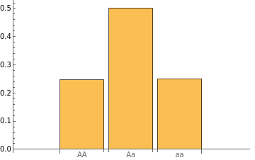
Offspring (-generation) therefore inherit one genetic allele from each Aa parent, and has one of three possible genotypes, AA, Aa(or aA), and aa.
F
2
In[2]:=
StringJoin@@@Tuples[{"A","a"},2]
Out[2]=
{AA,Aa,aA,aa}
In[3]:=
f2=Table[StringJoin[RandomChoice[{"A","a"}],RandomChoice[{"A","a"}]],{i,100000}];BarChart[{Count[f2,"AA"],Total[Count[f2,#]&/@{"Aa","aA"}],Count[f2,"aa"]}/100000,ChartLabels{"AA","Aa","aa"}]
Out[4]=
Law of Independent Assortment (the “Second Law”):
Law of Independent Assortment (the “Second Law”):
Genes for different traits assort independently of one another in the formation of gametes.
◼
For two different traits (A/a and B/b), each on a different pair of genes, there are four possible types of gametes.
In[5]:=
StringJoin@@@Tuples[{{"A","a"},{"B","b"}}]
Out[5]=
{AB,Ab,aB,ab}
◼
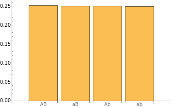
With the two pairs of genes, both parents produce 25% each of AB, Ab, aB, and ab for 100000 random gametes.
In[6]:=
gamete=Table[StringJoin[RandomChoice[{"A","a"}],RandomChoice[{"B","b"}]],{i,100000}];BarChart[Counts[gamete]/100000,ChartLabels{"AB","aB","Ab","ab"}]
Out[7]=
◼
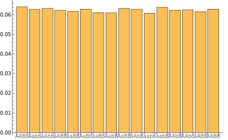
For AaBb x AaBb, each parent produces four different types of gametes and these gametes combine with each other in =16 different ways.
2
4
In[8]:=
TableForm[{{AABB,AaBB,AABb,AaBb},{AaBB,aaBB,AaBb,aaBb},{AABb,AaBb,AAbb,Aabb},{AaBb,aaBb,Aabb,aabb}},TableHeadings{{AB,aB,Ab,ab},{AB,aB,Ab,ab}}]
Out[8]//TableForm=
AB | aB | Ab | ab | |
AB | AABB | AaBB | AABb | AaBb |
aB | AaBB | aaBB | AaBb | aaBb |
Ab | AABb | AaBb | AAbb | Aabb |
ab | AaBb | aaBb | Aabb | aabb |
◼
It can be experimentally(computationally) shown.
In[9]:=
gamete1=Table[StringJoin[RandomChoice[{"A","a"}],RandomChoice[{"B","b"}]],{i,100000}];gamete2=Table[StringJoin[RandomChoice[{"A","a"}],RandomChoice[{"B","b"}]],{i,100000}];ff2=Table[StringJoin[StringTake[gamete1[[i]],1],StringTake[gamete2[[i]],1],StringTake[gamete1[[i]],{2}],StringTake[gamete2[[i]],{2}]],{i,100000}];DeleteDuplicates[ff2]
Out[12]=
{AABb,Aabb,aAbb,aABB,aaBB,AaBb,aaBb,AabB,AaBB,aAbB,aabb,aabB,AAbB,AAbb,aABb,AABB}
In[13]:=
BarChart[Counts[ff2]/100000,ChartLabelsAutomatic]
Out[13]=
Law of Dominance (the “Third Law”):
Law of Dominance (the “Third Law”):
Some alleles (A or B) are dominant while others (a or b) are recessive; an organism with at least one dominant allele will display the effect of the dominant allele. For example, when the dominant trait is red and the recessive trait is white, AA and Aa are red, and aa is white.
◼
The phenotypes of self-fertilization of F1-generation(Aa) show a 3(red):1(white) ratio in the F2 generation.
In[14]:=
BarChart{Count[f2,"AA"]+Total[Count[f2,#]&/@{"Aa","aA"}],Count[f2,"aa"]},ChartStyle{Red,White},ChartLabelsCallout[{"3","1"},Automatic],ChartLegends"AA or Aa\n"
,"aa\n"
Out[14]=
◼
For the AaBb parents (A: yellow(dominant), a: green(recessive), B: Round(dominant), b: wrinkly(recessive)), the phenotypes of two independent traits show a 9(yellow,round):3(green,round):3(yellow,wrinkly):1(green,wrinkly) ratio in the -generation.
F
2
In[15]:=
gen1=Total[Count[ff2,#]&/@{"AABB","AABb","AAbB","AaBB","AaBb","AabB","aABB","aABb","aAbB"}];gen2=Total[Count[ff2,#]&/@{"aaBB","aaBb","aabB"}];gen3=Total[Count[ff2,#]&/@{"AAbb","Aabb","aAbb"}];gen4=Total[Count[ff2,#]&/@{"aabb"}];BarChart{gen1,gen2,gen3,gen4},ChartStyle"Pastel",ChartLabelsCallout[{"9","3","3","1"},Automatic],ChartLegends
,
,
,
Out[19]=
◼
For each trait, the phenotypes show a 3(dominant):1(recessive) ratio in the -generation, confirming the independent assortment.
F
2
In[20]:=
BarChart{gen1+gen3,gen2+gen4}100000,ChartLabelsCallout"Yellow\n
","Green\n
",Top,BarChart{gen1+gen2,gen3+gen4}100000,ChartLabelsCallout"Round\n
","Wrinkly\n
",Top
Exception - Polygenic Inheritance
Exception - Polygenic Inheritance
Polygenic inheritance refers to a single trait that is controlled by the combined effect of more than one pair of genes while Mendelian traits can be traced on a single locus. Examples of human polygenic inheritance are height, skin color, eye color and weight.
Example: Skin Color
Example: Skin Color
For the simplification, we assume that three pairs of genes (A/a, B/b, C/c) control the skin color, and the capital letter genes (A, B and C), neither dominant nor recessive, add dark pigmentation as more melanin is produced.
◼
In the cross between two mulatto genotypes (AaBbCc x AaBbCc), the offsprings contain seven different shades of skin color based on the number of capital letters (0-6) in each genotype.
◼
For AaBbCc x AaBbCc, each parent produces eight different types of gametes and these gametes combine with each other in 64 different ways resulting in a total of seven skin colors.
◼
The distribution of phenotypes (7 skin colors) of offsprings can be calculated by probabilities.
Distribution of Phenotypes in Polygenic Inheritance
Distribution of Phenotypes in Polygenic Inheritance
By increasing the number of genes controlling a trait, the number of phenotype combinations also increase, until the number of phenotypes to which an individual can be assigned are no longer discrete, but continuous. Thus, polygenic inheritance patterns normally follow a normal (bell-shaped) distribution curve.
◼
As the number of genes controlling a trait increases, the distribution is more likely to follow a normal distribution curve.
Further Explorations
Heredity
Non-Mendelian inheritance
Incomplete dominance
Multiple Allele
Authorship information
Nae Eoun Lee
2017/06/23
nl2287@mit.edu


