Pigeonhole Principle
Pigeonhole Principle
A simple counting argument with great power
History
History
The Pigeonhole Principle is attributed to Peter Gustav Lejeune Dirichlet and its premise is of common sense. Nonetheless, this seemingly trivial revelation is a powerful tool in combinatorics as well as proving strong statements about collections without having to consider each element of a collection.
Definition
Definition
Let n and k be positive integers, and let n > k. Suppose we have to place n identical balls into k identical boxes, where n > k. Then there will be at least one box in which we place at least two balls.
Example:
Example:
Aside: Integer Partition
Aside: Integer Partition
We will use the function IntegerPartitions to "distribute" the number of balls into the exact number of boxes, by partitioning the integer balls into exactly {boxes} parts.
To give an example of an integer partition see that IntegerPartitions[4] yields a list of lists containing integers were the sum of those integers is 4.
To give an example of an integer partition see that IntegerPartitions[4] yields a list of lists containing integers were the sum of those integers is 4.
In[58]:=
IntegerPartitions[4]
Out[58]=
{{4},{3,1},{2,2},{2,1,1},{1,1,1,1}}
The latter can be showed by applying the function Plus to each sublist that is returned by IntegerPartitions[4].
In[99]:=
Plus@@@IntegerPartitions[4]
Out[99]=
{4,4,4,4,4}
Thus we see that an integer partition of the integer n into a list of length k is equivalent as distributing n balls into k boxes. Using the optional argument {k} we can specify that we want integer partitions of exactly k parts.
Applying the Pigeonhole Principle
Applying the Pigeonhole Principle
◼
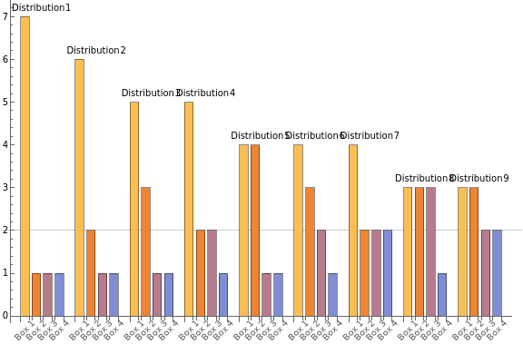
Here we will see that if we try to distribute10 balls amongst 4 boxes, then there will at least be a box with at least 2 balls.
In[324]:=
balls=10;boxes=4;
◼
Using IntegerPartition (as described above) we can find all the ways to distribute 10 balls amongst 4 boxes
In[353]:=
distributions=IntegerPartitions[balls,{boxes}]
Out[353]=
{{7,1,1,1},{6,2,1,1},{5,3,1,1},{5,2,2,1},{4,4,1,1},{4,3,2,1},{4,2,2,2},{3,3,3,1},{3,3,2,2}}
◼
Visualize the distribution of balls in boxes with a BarChart
In[326]:=
BarChart[distributions,GridLines{{},{2}},(*makeiteasiertoseeboxeswithatleast2ballsinthem*)ChartLabels{Placed[Table["Distribution "<>ToString[i],{i,Length@distributions}],Above],(*enumeratethedistributionpossibilities*)Placed[Table["Box "<>ToString[i],{i,boxes}],Axis,Rotate[#,Pi/4]&](*enumeratetheboxesofthedistributions*)},ImageSizeLarge]
Out[327]=
When n >> k such a bar chart will be unpractical to look at. Let us use AllTrue to show that the max value for each possible way to distribute the balls amongst boxes is in fact greater than or equal to 2!
In[61]:=
AllTrue[IntegerPartitions[balls,{boxes}],Max[#]≥2&]
Out[61]=
True
Generalized Definition
Generalized Definition
Let n, m and r be positive integers so that n > r • m. Let us distribute n identical balls into m identical boxes. Then there will be at least one box in which we place at least r + 1 balls.
Using this generalization we can see that the first definition was the case where r = 1. r can be thought as the replicate threshold for how many balls each box will at least have.
◼
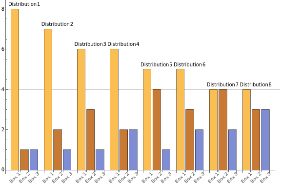
Here we will see that if we try to distribute10 balls amongst three boxes with a replicate of 3, then there will at least be a box with at least 4 balls.
In[354]:=
balls=10;boxes=3;replicates=3;
◼
As before we can enumerate all set of all ways to distribute the balls into boxes
In[357]:=
distributions=IntegerPartitions[balls,{boxes}];
In[358]:=
BarChart[distributions,GridLines{{},{replicates+1}},(*highlightwherer+1islocatedat*)ChartLabels{Placed[Table["Distribution "<>ToString[i],{i,Length@distributions}],Above],Placed[Table["Box "<>ToString[i],{i,boxes}],Axis,Rotate[#,Pi/4]&]},ImageSizeLarge]
Out[358]=
When n >> rm such a bar chart will be unpractical to look at. Let us use AllTrue to show that the max value for each possible way to distribute the balls amongst boxes is in fact greater than or equal to replicates + 1!
In[66]:=
AllTrue[IntegerPartitions[balls,{boxes}],Max[#]≥replicates+1&]
Out[66]=
True
Examples
Hair-raising power of the Pigeonhole Principle
Hair-raising power of the Pigeonhole Principle
Utilizing the Pigeonhole Principle we can prove that in New York City (NYC) there are at least two non-bald people with the same number of hair strands without having to hand count the strands on every individual’s head!
◼
First let us identify the number of people living in NYC as well as the maximum number of hairs on the human head
In[2]:=
population=hairs=Max
Out[2]=
Out[3]=
150000
To show that at least two people in NYC have the same number of hair strands, we must confirm that there are at least 150,000 + 1 people in NYC who are not bald.
◼
Using WolframAlpha we can figure out how many Americans have baldness
In[69]:=
WolframAlpha["Baldness","PodCells"][[3]]WolframAlpha["Baldness",{"Basic:DiseaseData","ComputableData"}][[1,2,2,-1]]
Out[69]=
| ||||||||||||||||||||
Thus we can calculate the number of non-bald people in NYC by using the pervasiveness of baldness and subtracting that percent from the populous.
As 8,543,453 is in fact greater than 150,000 it follows from the Pigeonhole Principle that there are at least two people with the same number of hair strands on their head.
Geometric Insights to data
Geometric Insights to data
The examples so far shows how we can prove strong statements without enumeration or comparison of all objects under consideration. This concept can also be utilized for understanding the geometric relationship of data.
Distance of Data Points
Distance of Data Points
◼
Generate ten random points within [0, 1]
Utilizing the Pigeonhole Principle we can prove that at least two of our points are closer than 0.48.
◼
Plot our data with grid lines showing the boxes
Then following the Pigeonhole Principle at least one box will contain at least two points (as 10 > 9).
Thus it follows that at least two points will be closer than 0.48!
We can also make a table of the distances between points and display in bold which points have a smaller distance than 0.48.
◼
The pairwise distances between points can easily be calculated by using DistanceMatrix.
Using a pattern we will display in bold which points have a smaller distance than 0.48.
Using a pattern we will display in bold which points have a smaller distance than 0.48.
Thus knowing only the domain and range of our data we can already identify some properties thereof.
Extension
Extension
We can further extend our insight to the spread of our data by changing r and m of the Pigeonhole Principle. For example, we can prove that with the same 10 data points that at least 3 of them are within a disk of radius 0.5.
◼
To prove the above statement we will divide - along the diagonals - our unit square into four “boxes”. Doing so, and applying the Pigeonhole Principle - it is clear that at least one box will contain 3 points.
To prove that the three points within such a region falls within a disk with radius 0.5, we need to get the circumcircle of one of the triangles. In this case we will use the bottom triangle (defined by the points {{0,1},{0.5,0.5},{1,1}})
◼
Plotting the triangle and circumcircle together we can see their relationship.
To get the radius of the disk which can contain the triangle we need to get the distance from one point at the boundary to the center. We will use the bottom left corner of the triangle ({0,0}) as this point.
Since at least three points will be in such a triangle, and the circumcircle around the triangle has a radius of 0.5 it follows that at least 3 points can be contained within a disk with radius 0.5.
Alternatively one can see that the a disk with radius 0.5 fits centered in the unit square also dividing the unit square into four parts (excluding the region inside the disk).
Assume the opposite (that three points are not within the disk above) then they must be within one of the four other regions. Again by the Pigeonhole Principle those 10 points must be within those four regions (and at least 3 are within one).
Calculating the area, it is clear that the area of any one of these regions is much smaller than the area of the disk and the proof follows
Calculating the area, it is clear that the area of any one of these regions is much smaller than the area of the disk and the proof follows
Further Explorations
Fubini Principle
Authorship information
Sumner Magruder
June 20th 2016
Mag.ds@live.com

