Approximations to the PrimePi Function
Approximations to the PrimePi Function
The PrimePi function(π[x]) shows the number of primes that are smaller than certain value x. Throughout history, there has been several approximation models of Prime-Counting function(π[x]). These models are important in that they reveal the long-term distribution of prime numbers (Prime Number Theorem, PNT) and help study various mathematical concepts such as LogIntegral and Big-O.
Distribution of Prime Numbers
Distribution of Prime Numbers
Let’s first look at the simple characteristic of prime numbers.
◼
Make a list of divisors for numbers from 2 to 10:
In[70]:=
Table[Divisors[n],{n,2,10}]
Out[70]=
{{1,2},{1,3},{1,2,4},{1,5},{1,2,3,6},{1,7},{1,2,4,8},{1,3,9},{1,2,5,10}}
Prime numbers are the ones that only have trivial divisors (i.e. 1 and itself). Thus, prime numbers have only 2 divisors.
◼
Select a list of divisors with length 2 for numbers from 2 to 10:
In[83]:=
Select[Table[Divisors[n],{n,2,10}],Length[Level[#,1]]2&]
Out[83]=
{{1,2},{1,3},{1,5},{1,7}}
Now let’s find the number of primes that are smaller than 100.
◼
Select prime numbers that are less than 100:
In[84]:=
Select[Table[Prime[n],{n,100}],#<100&]
Out[84]=
{2,3,5,7,11,13,17,19,23,29,31,37,41,43,47,53,59,61,67,71,73,79,83,89,97}
◼
Here is the number of primes that are less than 100:
In[85]:=
Length[Select[Table[Prime[n],{n,100}],#<100&]]
Out[85]=
25
Let’s now look at the distribution of primes by looking at the number of primes that are smaller than .
k
10
◼
Make a table of values with columns , number of primes smaller than , and frequency of primes under :
k
10
k
10
k
10
In[41]:=
Grid[Join[{{"n","PrimePi[n]","frequency"}},Table[{n,PrimePi[n],Round[PrimePi[n]/n,0.001]},{n,Table[10^k,{k,2,14}]}]],AlignmentLeft]
Out[41]=
n | PrimePi[n] | frequency |
100 | 25 | 0.25 |
1000 | 168 | 0.168 |
10000 | 1229 | 0.123 |
100000 | 9592 | 0.096 |
1000000 | 78498 | 0.078 |
10000000 | 664579 | 0.066 |
100000000 | 5761455 | 0.058 |
1000000000 | 50847534 | 0.051 |
10000000000 | 455052511 | 0.046 |
100000000000 | 4118054813 | 0.041 |
1000000000000 | 37607912018 | 0.038 |
10000000000000 | 346065536839 | 0.035 |
100000000000000 | 3204941750802 | 0.032 |
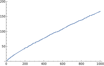
To see the distribution of prime numbers, let’s look at how the number of primes change with respect to positive integer n.
◼
Make a plot of PrimePi function:
In[91]:=
Plot[PrimePi[n],{n,0,1000},PlotRange{0,200}]
Out[91]=
First Approximation to the PrimePi Function
First Approximation to the PrimePi Function
Looking at how PrimePi function changes with n, let’s now find out the general pattern which the function contains. Lets look and the ratio of n to PrimePi[n].
◼
Make a table of values with columns and the ratio of numbers to their PrimePi:
k
100
In[40]:=
Grid[Join[{{"n","n/PrimePi[n]"}},Table[{n,Round[n/PrimePi[n],0.001]},{n,Table[10^k,{k,2,14,2}]}]],AlignmentLeft]
Out[40]=
n | n/PrimePi[n] |
100 | 4. |
10000 | 8.137 |
1000000 | 12.739 |
100000000 | 17.357 |
10000000000 | 21.975 |
1000000000000 | 26.59 |
100000000000000 | 31.202 |
If we look at the right column, we can find out that the numbers increase somewhat linearly.
◼
Find out differences between the values of ratio of n to PrimePi[n]:
In[99]:=
Differences[Table[Round[n/PrimePi[n],0.001],{n,Table[10^k,{k,2,14,2}]}]]
Out[99]=
{4.137,4.602,4.618,4.618,4.615,4.612}
We saw that the ratio of n to PrimePi[n] increases about 4.6 (more specifically, 4.60 to 4.62) for high values n. Let’s now reconsider how we set the left columns of the table above by looking at the logarithmic values.
◼
Find out differences between the logarithmic values of :
k
100
In[100]:=
Differences[Log[10,Table[10^k,{k,2,14,2}]]]
Out[100]=
{2,2,2,2,2,2}
These results are surprising since there is somewhat a linear relationship between and the ratio of numbers to their PrimePi. Considering such relationship, Carl Friedrich Gauss came up with the following approximation model in 1792.
Log[]
k
100
◼
Gauss’ first Approximation model:
In[101]:=
Framed"π(N)~"
N
Log[N]
Out[101]=
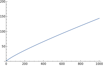
Let’s look at how the approximation model is plotted.
◼
Make a plot of :
N
Log[N]
In[102]:=
Plot[n/Log[n],{n,0,1000},PlotRange{0,200}]
Out[102]=
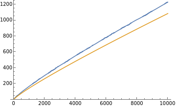
Let’s now compare Gauss’ first approximation model with the actual PrimePi function.
◼
Make a plot of and PrimePi[N] and :
N
Log[N]
In[103]:=
Plot{PrimePi[n],n/Log[n]},{n,0,10000},PlotRange{0,1250},PlotLegends"π[N]",""
N
Log[N]
Out[103]=
◼
Make a plot of absolute error of the approximation model :
N
Log[N]
In[105]:=
ListPlot[Table[Abs[(PrimePi[n]-n/Log[n])],{n,2,1000}]]
Out[105]=
◼
Make a plot of relative error of the approximation model :
N
Log[N]
◼
Make a table of values comparing nth prime number, the approximation nLog[n], and the relative error:
LogIntegral Function
LogIntegral Function
The above graph goes to -∞ when n is 0, becomes 0 when n is about 1.45137, and increases afterwards.
◼
Find a value(nonzero) that makes the LogIntegral[n] 0:
◼
Improved Approximation model:
Let’s look at how the improved approximation model is plotted.
◼
Make a plot of Li[n]:
Let’s now compare the improved approximation model with the first approximation model and the actual PrimePi function.
◼
Make a plot of absolute error of the approximation model Li[N]:
◼
Make a plot of relative error of the approximation model Li[N]:
Further Improvements
Further Improvements
Although Li[N] is a very strong approximation model for the PrimePi function, mathematicians consistently tried to make even better models for the PrimePi function. One of the examples is the usage of asymptotic expansion in Li[N].
◼
Refined Approximation model using asymptotic expansion:
Let’s look at how the approximation model using asymptotic expansion is plotted.
Let’s now compare the approximation model using asymptotic expansion, Li[N], and the actual PrimePi function for large numbers.
◼
Riemann’s refined approximation model:
Let’s look at how Riemann’s refined approximation model is plotted.
Let’s now compare Riemann’s refined approximation model, Li[N], and the actual PrimePi function for large numbers.
With the above developments and researches related to Riemann Hypothesis, Helge von Koch finally made a model in 1901 that equates PrimePi function with a set of equations assuming that Riemann Hypothesis is true (It has still not been proven: http://mathworld.wolfram.com/RiemannHypothesis.html).
◼
Koch’s Result:
Further Explorations
Investigate the relationship between PrimePi function and Riemann Hypothesis
Investigate the Big-O value for each number and make better approximation model
Authorship information
Sung Min Yoon
2017/06/23
sy375@cornell.edu


